Imagine this
A radio signal gets weaker as it travels. Walls and weather can change it. The listening radio needs enough signal to hear the message.
THE FIELD GUIDE / 009 · RADIO PROPAGATION
Radio links depend on a path, enough signal and a receiver that knows what to listen for.
Explore four separate questions: how a wave spreads, what the ionosphere can change, how long travel takes and what noise a receiver admits. The calculations below teach mechanisms; they do not predict coverage for a real station.
Explore distance and frequency ↓A radio signal gets weaker as it travels. Walls and weather can change it. The listening radio needs enough signal to hear the message.
Radio link calculations help reason about distance, atmosphere, antennas and receiver noise. A real link plan needs local measurements.
The calculations use specified conditions; terrain, interference, weather, pointing and hardware can change real performance.
Read-aloud starter; not yet tested with children. The fuller science, data, figures and sources follow below.
01 / SPREADING IS NOT ABSORPTION
Imagine a lamp illuminating a larger and larger sphere. Its power is spread over more area. A radio antenna also intercepts only part of a spreading wave. In empty space this geometric effect exists even when nothing absorbs the wave.
Both sliders use logarithmic scales: equal steps multiply the value. Frequency counts cycles per second; one MHz is one million cycles per second.
Try this: compare 100 MHz at 1 km and 10 km. Ten times the distance adds 20 dB of loss: a hundredfold power reduction for the same antenna gains.
λ = c/f · L = 20 log₁₀(4πdf/c)
Use metres, hertz and c = 299,792,458 m/s. The loss compares power for ideal isotropic antennas; actual antenna gains are added separately. This comparison holds dimensionless antenna gains fixed. A fixed-size receiving dish has a frequency-dependent gain, so changing frequency with the same dish is a different comparison.
Assumptions: unobstructed far field, free space and matched polarization. No terrain, Earth obstruction, rain, atmospheric absorption or multipath. These hypothetical path lengths are not distances along the ground. Higher frequency does not travel faster in vacuum.
| Distance (km) | Loss (dB) | One-way delay (ms) |
|---|
02 / DIFFERENT PATHS, DIFFERENT CONDITIONS
A direct path can connect nearby antennas or an antenna and a spacecraft. Ground-related propagation depends on the surface and frequency. A sky wave bends through a changing ionized atmosphere; it does not bounce off a solid mirror.
HF is the 3–30 MHz band commonly associated with ionospheric links. These band names are conventions, not promises: reception also depends on time, path, absorption, antennas and interference. Geometry alone cannot tell us whether a message will be readable.
03 / A DELIBERATELY SIMPLE IONOSPHERE
Sunlight can free electrons from atmospheric atoms and molecules. Their collective response changes how radio propagates. In a simplified layer, the peak electron density sets a vertical critical frequency. The model below ignores Earth's magnetic field and collisions.
0° points upward; a larger angle is more oblique. This is the angle where the refractive index is approximately one, below the ionosphere, not the local angle where a ray turns.
Try 60°: the flat-layer relation doubles the vertical frequency. This does not establish a usable real-world link. Even a frequency below the ideal limit may be absorbed or too weak to decode.
fₚ = √(nₑe²/(ε₀mₑ))/(2π) · f = f꜀/cos(θ₀)
Electron density nₑ is in electrons per cubic metre. The plasma model is cold, collisionless and unmagnetized, with stationary ions. The secant relation assumes a flat, horizontally uniform, stratified layer; f꜀ is its equivalent vertical critical frequency.
The slider stops at 75° as a teaching limit, not a validated operational boundary. Extending the flat formula toward 90° would diverge; that is not unlimited real-world communication. Earth curvature, density profiles, geomagnetic modes, absorption, scattering and changing conditions require additional modelling. The diagram above is not a ray trace.
04 / WAITING IS NOT MESSAGE LENGTH
This uses the path length selected in the first experiment. A message that takes one second to send still takes one second to receive in this stationary vacuum example. Both ends of it are shifted in time.
At 1,000 km, one-way vacuum delay is about 3.336 milliseconds. A separate pulse returned over the same fixed path with 0.2 seconds of turnaround arrives about 0.206671 seconds after transmission.
One-way geometric delay is d/c. A symmetric stationary round trip is 2d/c plus turnaround. For a reply that waits for the entire message, its duration must also be included. Moving endpoints, different outbound and inbound paths, plasma group delay and processing require a more complete model.
A recording's duration does not tell us how far it travelled. A light-year is a distance: converting it to vacuum travel time follows its definition, rather than independently measuring a source.
05 / A RECEIVER MUST MATCH THE TASK
A receiver selects a band of frequencies. Widening it admits more broadband noise; narrowing it too far can remove useful parts of the waveform. This calculation isolates one contribution: a matched thermal source at 290 K.
Noise power N = kTB
Choose a suitable antenna, orientation and polarization. Account for cable losses, pointing and the receiving environment.
Specify tuned band, equivalent noise bandwidth, interference, calibration and adequate sampling. Receiver electronics add noise too.
Specify modulation, symbol timing, coding and decision rules. Detecting energy is not decoding bits, interpreting them or locating a sender.
A tenfold bandwidth increase adds 10 dB of thermal noise here. It does not by itself give a bit-error probability. Explore a specified modulation and detector in Sending information reliably.
06 / REPRODUCIBLE PARAMETER STUDY
632 ANALYTICAL CALCULATION ROWS · NOT MEASURED RECEPTION
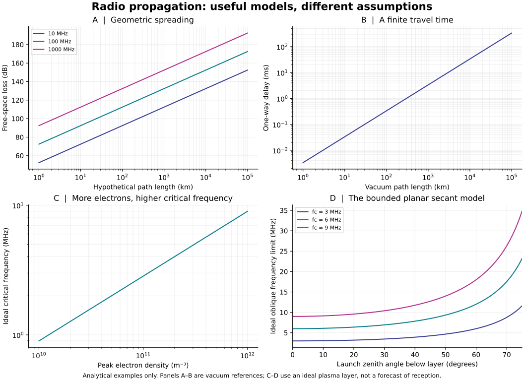
Run generate.py with Python, NumPy and Matplotlib. The 303 free-space rows cover 101 distances and three frequencies; 101 rows vary electron density; 228 rows cover 76 angles and three vertical critical frequencies. An independent flux-times-effective-aperture derivation checks the loss values. Scaling checks test doubling distance and frequency, quadrupling electron density and known angles.
07 / WHAT THIS CAN IMPROVE
A remote sensor link can fail because of obstruction, poor antenna orientation, interference, timing or insufficient signal. More transmitter power addresses only some of those causes.
For distant control, distinguish travel delay from message duration and processing. For ionospheric links, consult measured conditions and a path-specific model rather than relying on this flat-layer example.
Record the path, antennas, waveform, power, bandwidth and intended error rate. Separate assumed values from measurements.
A proposed receiver study would compare calibrated signal and noise over the same band, then measure errors using known test messages. No such hardware trial is reported here.
Repeat under documented conditions and retain failures. A plausible path and a computed delay do not independently verify an unrecorded reception.
READ FURTHER
ITU-R P.525 · Free-space attenuation provides the spreading-loss framework.
BIPM · The metre defines the exact vacuum speed used for wavelength and delay.
NOAA · HF radio communications explains how ionospheric conditions affect radio paths.
NASA DSN Module 214, Revision B · PN ranging discusses travel-time measurements and moving geometry.
NASA · Small spacecraft communications describes antenna, receiver and link-design constraints. The downloadable methods file includes the plasma, secant-law and physical-constant references.
Revised 27 September 2026. All interactive results are conditional teaching calculations; no actual radio reception or coverage is validated.
The ionosphere affects radio through its free electrons. In the lower atmosphere, changes in the air’s refractive properties can bend a radio path: this is refraction. Some atmospheric profiles can guide propagation within a layer, called ducting; irregularities can also redirect some energy through scattering. These are distinct mechanisms, not one universal atmospheric mirror.
ITU: tropospheric refraction · ITU: propagation mechanisms (2015 edition) · NOAA: the ionosphere.
Hearing a weak, distant station does not identify the path that carried its signal. Comparing explanations needs the frequency, transmitter and receiver locations and heights, atmospheric conditions and recorded signal behavior. This page’s ionosphere slider does not calculate tropospheric refraction, ducting or scattering. No particular mechanism is established for the unrecorded reception described in the proposal.