Imagine this
A room may have enough space in total but still be too small for one big thing. A schedule can share time between machines. People must choose what matters and what is fair.
THE FIELD GUIDE / 034 · OPTIMIZATION AND DECISIONS
A computer can have spare processing power and still reject a job because its memory is full. A satellite can see a region for longer from a higher orbit while losing fine detail. Better planning starts by making competing limits visible.
Try fitting a job ↓A room may have enough space in total but still be too small for one big thing. A schedule can share time between machines. People must choose what matters and what is fair.
Capacity and scheduling models help compare whether jobs fit and where bottlenecks occur. A real planner needs agreed goals and constraints.
The page's optimization examples do not establish a real-world best or permitted policy; costs, capacity, preferences and consequences need evidence and human choices.
Read-aloud starter; not yet tested with children. The fuller science, data, figures and sources follow below.
Imagine two computers. Each offers 100 abstract units of processing capacity and 64 GB of memory. A new job must fit both its requirements on the same computer. Adding up free resources across the room can hide a bottleneck.
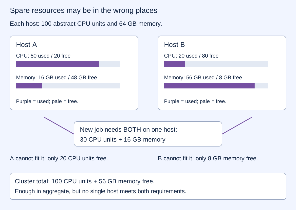
Admission decides which requests to accept. Placement decides where they go. Scheduling decides when they run. Priorities and fairness decide whose request waits. These are related questions, not interchangeable answers.
FIXED SNAPSHOT · NO JOB IS ACTUALLY RUN
Existing use is fixed: A uses 80 CPU units and 16 GB; B uses 20 CPU units and 56 GB. Change the new request. The checks below do not reserve resources or rearrange existing jobs.
| Host | Free CPU units | Free memory (GB) | Result |
|---|
Try 20 CPU units and 16 GB: A can accept it. Try 30 CPU units and 8 GB: B can accept it. A larger system also needs reliable inventories, concurrent reservation checks, handling for failed machines and a policy that does not indefinitely postpone some requests.
The Borg cluster-management paper describes established admission, placement and sharing methods. This small puzzle is not a reproduction or benchmark of that system.
HYPOTHETICAL POWER AND THERMAL MODEL
Split the same assigned CPU load evenly across one to five identical hosts. In this example, heavily loaded hosts draw disproportionately more power. Spreading the load can reduce that part of the bill, but every powered host also consumes 70 W before doing useful work.
The time slider changes only the thermal response. The energy comparison always covers 60 seconds. The table compares the same assigned load; it does not measure completed jobs, throughput, response time or service quality.
| Hosts sharing load | CPU per selected host | IT power (W) | Facility energy, 60 s (kJ) | Selected host temperature (°C) |
|---|
Each host has 100 CPU units of capacity. For total load L spread over n hosts, utilization u=L/(100n). Reject a choice if L>100n. Assigned per-host power is P=70+180u² W. Total IT power is nP plus 70 W for each remaining powered host. Facility power is 1.30 times IT power; multiplying by 60 seconds gives energy in joules.
The temperature model uses ambient and initial temperature 25 °C, thermal resistance 0.1 K/W and time constant 300 s. Under constant host power P, T(t)=25+0.1P[1−exp(−t/300)]. This is the exact response of the declared first-order model; its parameters are hypothetical. It approaches a finite equilibrium rather than adding the full steady-state rise at every time step.
The corresponding interval update is Tnext=25+(T−25)exp(−Δt/300)+0.1P[1−exp(−Δt/300)]. An earlier project calculation omitted the final bracketed factor. These new calculations correct that model and do not reuse its performance claims. Historical files remain preserved separately.
Real processors do not necessarily follow this quadratic law. Switching hosts off takes time and may cost energy; redundancy, memory placement, deadlines and cooling dynamics constrain real choices. The fixed 1.30 facility multiplier is not a cooling-system simulation. The thermal output is not a safety rating. At zero load the selected hosts still draw idle power, and energy per unit of assigned load is undefined.
A lower circular orbit gives an ideal camera a smaller diffraction separation scale near the point directly below it. A higher orbit can give a longer view of a stationary target during a central pass. Neither benefit automatically decides which orbit is preferable.
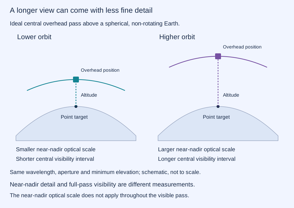
A candidate is dominated if another is at least as good on both chosen objectives and strictly better on one. Non-dominated candidates form a tradeoff frontier. That does not make them practical or supply a single winner.
19 SAMPLED CIRCULAR ORBITS · ASSIGNED REQUIREMENTS
The camera wavelength is 550 nm and aperture diameter 0.10 m. Visibility means a central pass above 30° elevation on a spherical, non-rotating Earth. All 19 sampled altitudes trade a smaller ideal optical scale against longer visibility; none dominates another on these two quantities.
| Altitude (km) | Near-nadir scale (m) | Visibility (s) | Period (min) | Current requirements |
|---|
For Earth radius R=6378.137 km, orbital radius r=R+h and gravitational parameter μ=398600.435507 km³/s², angular speed n=√(μ/r³). At minimum elevation e=30°, the central half-angle is ψ=acos[(R/r)cos(e)]−e. Visibility duration is 2ψ/n; period is 2π/n. Angles are calculated in radians.
The near-nadir Rayleigh separation scale is 1.22λh/D, with wavelength λ, altitude h and aperture diameter D expressed in metres. It is not detector ground sample distance, and it is not maintained throughout the visibility interval. Pixel size, atmosphere, pointing, contrast, exposure, slant range and projection require further analysis.
The starting limits of 5 m and 120 s are invented teaching requirements. They select 300–700 km in this sampled grid. Other altitudes between grid points have not been enumerated here. This is not a pass predictor for a location, date or orbit inclination; Earth rotation and non-central passes are omitted.
A machine may have enough capacity to perform an action while a mission rule forbids it. Keep three questions separate: can the equipment do it, are resources available, and is the action authorized? A numerical score cannot settle the last question.
These examples contain no operational intervention or travel policy. Real planning must define resource reservations, failure handling, safety margins and authorization independently. Mission risk and an option to withdraw are additional requirements; neither is quantified by this optical-and-visibility comparison. A copied permission record or a successful calculation is not a new permission.
Today: shared compute queues, laboratory bookings and observation planning benefit from explicit demands, refusals and competing objectives. A well-chosen rule can make available capacity more useful, but its value must be checked against the work actually delivered.
A possible next step: compare candidate policies against measured workloads, calibrated power curves and agreed fairness and reliability requirements. Include delays, rejected requests, cooling and recovery from failures. No new scheduler or quantified real-world saving is established by this chapter.
REPRODUCIBLE TEACHING STUDY
The downloadable study keeps the corrected hypothetical power/thermal model separate from the historical scheduler. Orbital calculations reproduce the declared circular geometry with corrected optical terminology. There are no new hardware measurements.
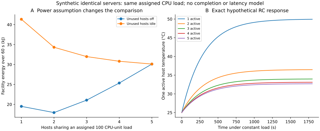
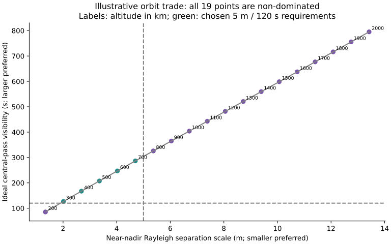
1,943 calculation rows: 1,010 energy cases, including 400 infeasible assignments with blank outputs; 905 thermal samples; 19 orbital candidates;9 optical sensitivity summaries. These counts do not express confidence or practical performance.
To reproduce, save the script and numeric reference together and run with Python, NumPy and Matplotlib. Reference values preserve the historical orbital calculation with neutral labels. The generator hash, runtime and reference provenance hashes are recorded. Independent ray/sphere geometry agrees with the visibility calculation within6×10−13s; the corrected thermal recurrence agrees with the closed-form solution. These numerical checks do not validate the hypothetical power law.
Conservation of capacity and consistent units come before any claim of improvement. Impossible CPU assignments remain marked, rather than silently dropping work. The power comparison fixes assigned load and duration. The orbital comparison reports all candidates and sensitivity to wavelength and aperture.
Google Research: Borg cluster management · NASA/JPL: astrodynamic parameters · NASA: gravity and mechanics
The references establish conventional methods and constants; they do not validate the assigned server power law or a specific mission. Full models would need measured execution, memory and network constraints, thermal coupling, orbital lifetime, communication, pointing and uncertainty.
A capacity check asks whether a job fits available resources. Crediting an account, approving a budget and promoting someone in a hierarchy are different decisions. They need stated rules, records and authorization; a person's identifier or a computer's ability to calculate does not establish that those decisions are justified.
Examine what a score establishes and check the supporting records.
Consider the proposed rule A = B/C². Holding B at 100, C = 2 gives A = 25; doubling C to 4 gives A = 6.25. The output falls by a factor of four, not two. The rule is undefined at C = 0. Before interpreting A as remuneration, we still need the units, scales and operational meanings of B and C. Correct arithmetic does not establish fair pay or a useful incentive. A computing-capacity model does not test that policy.
C₀ is a positive reference coefficient and A₀ is its corresponding output, with B held fixed. The solid curve follows the squared-denominator equation. The dashed curve is a separately normalized inverse-linear comparison: the accompanying description suggests this different rule. Comparing the curves does not settle which policy was intended.
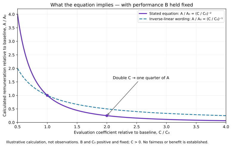
| Coefficient C/C₀ | Squared rule A/A₀ | Linear comparison |
|---|---|---|
| 0.5 × reference | 4 | 2 |
| 1 × reference | 1 | 1 |
| 2 × reference | 0.25 | 0.5 |
| 4 × reference | 0.0625 | 0.25 |
Download the 141 calculated rows · Reproduce the figure
To reproduce the downloads, install Python and Matplotlib, then run the downloaded script. It writes the CSV data and SVG and PNG figures beside the script.