Imagine this
A quiet signal can hide inside noise. We choose a rule for when it is strong enough to notice. A more permissive rule may find more signals but also make more mistakes.
THE FIELD GUIDE / 004 · SIGNALS
Turn up the threshold and fewer false alarms get through. But what else do you miss?
A detector needs a rule for deciding when a reading is unusual enough to investigate. A stricter rule can reject noise and real signals alike. Searching in more places creates another trade-off.
Set the threshold ↓A quiet signal can hide inside noise. We choose a rule for when it is strong enough to notice. A more permissive rule may find more signals but also make more mistakes.
Detection rules help teams compare missed signals with false alarms. A detector for a particular task needs representative test data.
The computer-made signals check that the calculation works; they do not give a general chance of finding a signal in the real world. A false alarm means saying “I found it” when it was not there.
Read-aloud starter; not yet tested with children. The fuller science, data, figures and sources follow below.
THE SIMPLE VERSION · NO MATHS NEEDED
Imagine a tiny bell ringing while people are talking. Sometimes the room makes a sound that only seems like the bell. A detector draws a line: if a reading is louder than the line, it asks someone to check.
Move the line higher and fewer ordinary noises trigger an alert, but you may miss a real quiet bell. Move it lower and you catch more quiet bells, but more random sounds get through. There is no perfect line for every job.
Why this can help: Clear thresholds help researchers and instrument teams decide which readings deserve a closer look, while keeping missed changes and false alerts visible.
The graph below is an ideal teaching model, not measurements from a detector. Try moving the threshold and compare the two kinds of mistake ↓
01 / EXPERIMENT
σ means one standard deviation of the noise. The detector flags scores above this line.
A stronger signal shifts the blue distribution to the right. Both distributions have the same width.
Independent opportunities for noise to cross the threshold. Overlapping windows are not automatically independent.
These probabilities come from equations, not a random sample or measured detector.
Pink dashed: noise only. Blue solid: signal present. Shaded areas to the right of the threshold are the corresponding probabilities. Curve height is probability density, not probability at one exact score.
02 / UNDERSTAND
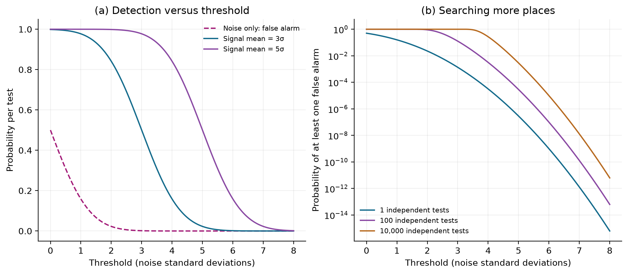
At a threshold of 3σ, a noise-only test crosses the line about 0.135% of the time. Repeat that test independently 1,000 times and the chance of at least one false alarm is about 74%.
That does not mean 74% of your candidates are false. The probability that a candidate represents a real signal also depends on how common real signals are and how well your model matches reality.
Raising it lowers false alarms but can hide weak signals. The right choice depends on the consequences of both kinds of mistake.
More frequencies, locations or times mean more opportunities to find an unusual noise fluctuation.
Repeat observations, independent sensors and background checks help distinguish a persistent effect from a statistical candidate.
03 / ANALYTICAL STUDY
IDEAL GAUSSIAN MODEL · 243 TABULATED SETTINGS · No measured performance claim
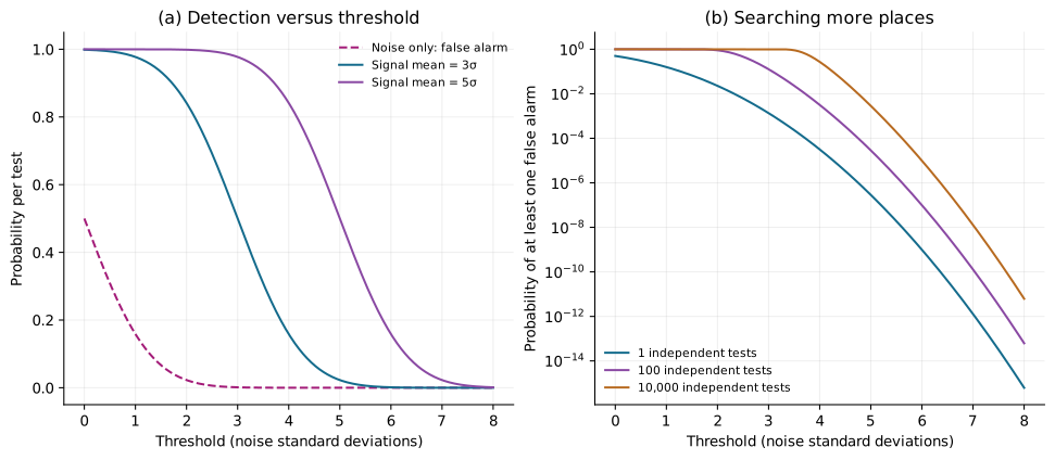
A 5σ threshold makes one noise fluctuation very unlikely. Across 10,000 independent tests, however, the chance of at least one crossing is about 0.286%. A signal with mean score 3σ crosses that same threshold only about 2.28% of the time.
| Threshold (σ) | Tests | Per-test false alarm | At least one false alarm |
|---|---|---|---|
| 3.0 | 1 | 0.0013499 | 0.0013499 |
| 4.0 | 1 | 3.16712e-05 | 3.16712e-05 |
| 5.0 | 1 | 2.86652e-07 | 2.86652e-07 |
| 3.0 | 100 | 0.0013499 | 0.126355 |
| 4.0 | 100 | 3.16712e-05 | 0.00316216 |
| 5.0 | 100 | 2.86652e-07 | 2.86648e-05 |
| 3.0 | 10000 | 0.0013499 | 0.999999 |
| 4.0 | 10000 | 3.16712e-05 | 0.271463 |
| 5.0 | 10000 | 2.86652e-07 | 0.00286241 |
Probabilities in this table range from 0 to 1; multiply by 100 for percentages.
Noise-only scores follow a standard normal distribution N(0,1). With a signal, scores follow N(A,1), where A is the selected mean signal score. The noise mean and variance are assumed known exactly. A score must exceed threshold τ.
With Q the upper standard-normal tail: false alarm = Q(τ), detection = Q(τ − A), and the chance of at least one false alarm across M independent noise-only tests is 1 − (1 − Q(τ))ᴹ. The expected number of false alarms is M Q(τ); unlike a probability, this can exceed one.
Python 3.12 with Matplotlib. The script writes results into signal-study beside itself. Browser probabilities use numerical Gaussian-tail integration, checked against the exported values.
Real noise may be correlated, non-Gaussian, drifting or contaminated by interference. A threshold calibrated under the wrong noise model can give misleading probabilities.
The family formula requires independent tests. With dependent tests and calibrated individual probabilities, the union bound gives an upper bound min(1, M p), not generally an equality. Detection here refers to the specified signal window, not the chance of choosing the correct maximum from an entire search.
A single injected signal at one location and several amplitudes can check a pipeline’s behaviour. It cannot by itself establish a general detection probability.
04 / WHAT THIS COULD IMPROVE
Compare missed events and false alerts before choosing a threshold for a monitoring system.
Record how many comparisons were made and which patterns were selected before looking at the data.
No detection only describes what the instrument searched for, when, and with what sensitivity. It does not rule out every possible signal.
A STRING, TWO ENDS, MANY PATTERNS
The simple version: Hold a skipping rope at both ends and shake it. Ripples travel away, bounce back, and overlap. For some shake rates, their combined motion makes a pattern that seems to stay in place: a few spots always stay still, while the parts between them move. Those still spots are called nodes.
A node is a place where this string’s sideways motion cancels. It is not a knot where extra material piles up. This familiar string example helps us understand waves; it does not show that waves create mass in the universe.
The model is loading.
Ideal model: y(x,t) = A sin(nπx/L) cos(2πfnt + φ), with λn = 2L/n and fn = n/(2L) √(T/μ). Here n is the mode, L the string length, T its tension, μ its mass per metre, and φ the starting phase.
This calculation assumes a uniform, perfectly flexible string under constant tension, small sideways motion, fixed ends and negligible damping. It is a mathematical illustration, not measured data or a model of the cosmos. In real strings, losses and construction affect the motion.
Why learn this? The same well-tested ideas help explain musical instrument tones and why engineers check structures for harmful resonance. They show how a clear model can guide useful measurements; they are not an application of the unverified mass claim.
Learn more: OpenStax, University Physics, “Standing Waves and Resonance” (superposition, fixed-end boundary conditions and allowed string modes).
05 / WAVES AND MEASUREMENTS
The same measurement ideas help explain phase cancellation, echoes, and how a software test can recover a deliberately added pattern. Each example answers a different question; none is proof of a particular source.
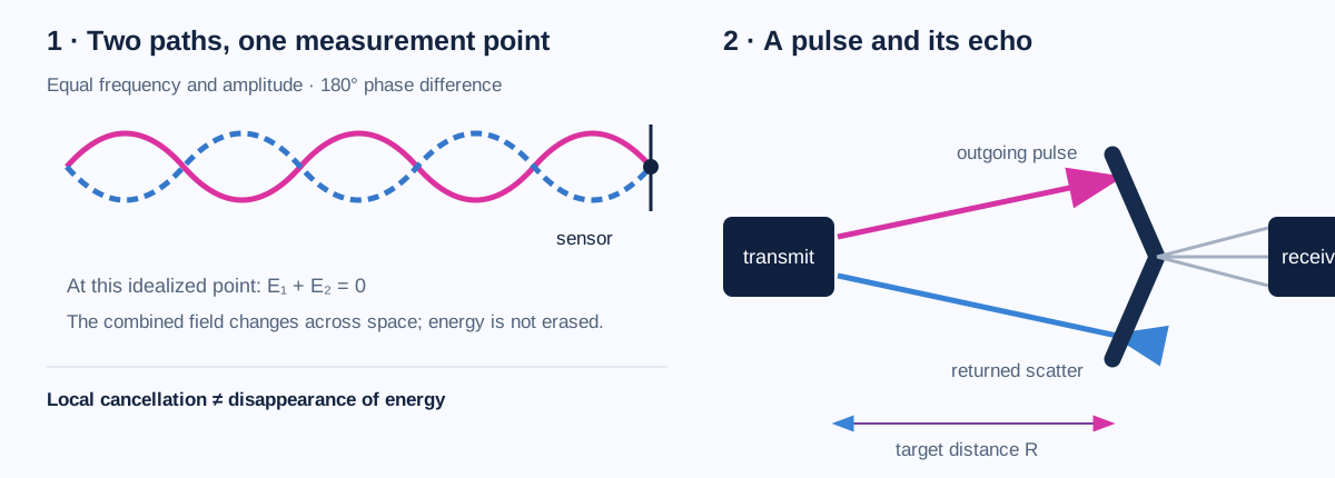
When two same-frequency waves arrive with equal amplitude and a half-cycle phase difference, their measured disturbances add to zero at that point. Move the sensor, change the path length, or change the phase and the result can change. The waves have reshaped the spatial pattern; the energy has not vanished. This is the ordinary superposition rule, not evidence for a new cosmological mechanism.
A transmitter sends a pulse; a surface scatters part of it; a receiver measures the returned signal. For a simple monostatic path, range is estimated as R ≈ cΔt/2, where Δt is the round-trip time and c is the propagation speed. That relation assumes the path and timing are known. Echo strength also depends on geometry, wavelength, polarization and material. This is a measurement lesson, not a claim that any particular object has a measured signature.
NASA/JPL · Radar measurement and backscatter · NASA · Synthetic-aperture radar geometry
REPRODUCIBILITY CHECK · PRESERVED LOCAL INPUT
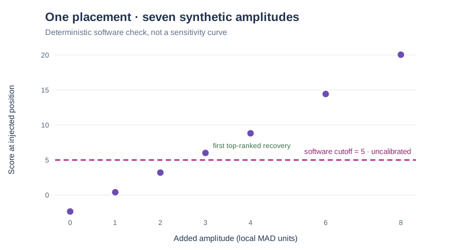
A small software check examined the first 12 complete spectra available in a preserved local filterbank prefix. It searched 512 channels using a stationary 8-frame template, with five possible start positions. Seven synthetic amplitudes were added to the same channel and same start position. The search first ranked the injected pattern highest at 3 local median-absolute-deviation (MAD) units.
| Added amplitude (local MAD units) | Score at injected position | Largest search score | Injection ranked first? |
|---|---|---|---|
| 0 | −2.4173 | 3.3454 | No |
| 1 | 0.3903 | 3.3454 | No |
| 2 | 3.1980 | 3.3454 | No |
| 3 | 6.0057 | 6.0057 | Yes |
| 4 | 8.8133 | 8.8133 | Yes |
| 6 | 14.4286 | 14.4286 | Yes |
| 8 | 20.0439 | 20.0439 | Yes |
What this shows: the code can recover a stationary synthetic line at this one tested placement and these amplitudes.
What it does not show: a detection-probability curve, a calibrated sensitivity, a measured false-alarm probability, Gaussian significance, performance on a new observation, a full-band search, or a search for drifting signals. The software's “5 sigma” threshold is not independently calibrated here; scores use local median/MAD normalization and overlapping windows. The 12 spectra are a bounded subset of 31 complete spectra in the retained prefix, not a full observation.
Provenance boundary: the retained 64 MiB input has SHA-256 0145871c…1265cc4; the analysis script and result hashes are in the downloadable methods JSON. The available record does not preserve an upstream download URL and independent archive checksum, so reacquisition of the exact input is not established.
READ FURTHER
NIST · Normal distribution explains the distribution used in this teaching model.
MIT · Signal detection in noise and the matched filter provides a broader introduction to detection methods.
NIST · Bonferroni’s method explains control of multiple comparisons. The independent-search formula above is a direct probability calculation under its stated assumptions.
Revised 28 September 2026. Original analytical teaching study; not a peer-reviewed detector evaluation.
A statistical detector does not test every physical explanation for a signal. See what a proposed wave model must define before it can be tested.