Imagine this
A camera can measure kinds of light our eyes cannot see. Plants, water and other materials can look different in different light. These clues do not always name exactly what is there.
THE FIELD GUIDE / 021 · SPECTRAL IMAGING
A spectrum can reveal differences our eyes miss. Learning what a detector actually measures helps turn those differences into useful evidence.
A camera can measure kinds of light our eyes cannot see. Plants, water and other materials can look different in different light. These clues do not always name exactly what is there.
Today, special cameras help map changes in plants, water and land. Extra colours of light might help tell materials apart in a particular place, but people must check samples from that place.
The page's example spectra are synthetic; different materials can look alike to a sensor. A match needs alternatives, calibration and other evidence.
Read-aloud starter; not yet tested with children. The fuller science, data, figures and sources follow below.
Two surfaces can look the same to our eyes and behave differently at another wavelength. A spectral camera compares selected parts of the electromagnetic spectrum. This can reveal useful differences, but every recorded band still needs an explanation: where did the radiation come from, what changed it, and what did the detector actually measure?
An ordinary colour image combines broad red, green and blue channels. A multispectral instrument measures several chosen intervals, sometimes outside visible light. An imaging spectrometer can sample many narrower intervals. Filters and detectors have response curves; they do not measure a perfectly isolated colour unless that is an explicit approximation.
Band choice matters. A narrow absorption feature may disappear when averaged with neighbouring wavelengths. More bands can help, but do not automatically solve noise, calibration or overlapping material signatures. Established uses include mapping vegetation, water and changes in land cover. NASA's Landsat band guide
SYNTHETIC EXPERIMENT
We invent two materials, A and B. They share a broad absorption feature; B has an extra narrow dip centred at 850 nm. These curves are mathematical examples, not mineral measurements. Choose how much of an unresolved pixel is covered by A, with B covering the rest.
The plotted curve is the assigned material property, even when illumination is off. The shaded interval is the band being averaged. The detector outputs below require illumination.
| Band | Normalized reflectance |
|---|
Broader bands dilute the narrow dip. Normalization against a reference under the same illumination makes the ideal reflectance independent of positive illumination strength. This does not mean a real detector works equally well in dim light: noise is absent here. At zero illumination, the normalization is undefined, not evidence for a black material.
The linear mixture assumes adjacent patches under common illumination and viewing conditions. It does not describe grains mixed inside a powder, multiple scattering or the abundance of a real mineral.
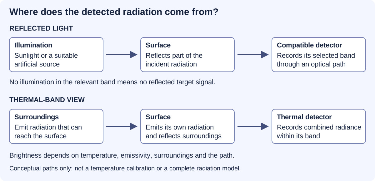
Reflected-light imaging needs illumination in the detected band. A scene can be dark to our eyes yet illuminated in near-infrared. A compatible camera can record that reflected light. Switching off all relevant illumination removes this reflected signal; greater sensitivity cannot create photons that never arrive.
Thermal imaging uses radiation emitted by surfaces. An object does not need a visible lamp to emit thermal infrared. But its measured brightness also depends on its surface properties, reflected surroundings and the path to the camera. A bright thermal pixel is not automatically a direct thermometer reading. NASA infrared explanation
Useful today: locating patterns consistent with heat loss or comparing surface conditions. Interpreting a temperature requires calibration and assumptions about the material and environment.
Near-infrared, thermal infrared and ultraviolet place different demands on detectors, filters and optics. Air also transmits some wavelengths much better than others. Extreme ultraviolet cannot be treated as ordinary light travelling freely across a room; specialised instruments manage the optical path and absorption. A frequency-to-wavelength conversion locates a band. It does not demonstrate a working camera. NASA/JPL UV instrumentation
Some minerals absorb more strongly in particular wavelength regions. Comparing an observation with measured reference spectra can suggest a material or mineral group. The USGS maintains such a reference collection. USGS Spectral Library
The match is rarely just a name lookup. One pixel may contain several materials. Dust can cover a surface, grain size can alter its spectrum, illumination can change, and the sensor may average away a useful feature. Different combinations can produce similar measurements. A spectral match should therefore be reported with alternatives and limitations, then checked against other evidence when the decision matters.
Useful today: narrowing a geological survey or choosing samples for closer analysis. A few colours do not establish an exact crystal structure. More detailed measurements can strengthen the interpretation, but their adequacy depends on the question.
PUBLISHED STUDY / READING A FAINT SIGNAL
The very simple version: Imagine listening to a quiet song behind a noisy fan. Removing the fan sound helps, but we must check that we have not changed the song. Scientists face a similar problem when they clean up a faint telescope signal.
WISE 0855 is a very cold brown dwarf. Its infrared spectrum provides a real example of how scientists check their measurements before interpreting an atmosphere. In 2020, Miles and colleagues processed the earlier observations again and compared the result with the reduction published by Skemer and colleagues in 2016.
Why this helps: reliable spectra can help us investigate the chemistry of distant atmospheres. The broader lesson also matters for measurements closer to home: conclusions should survive checks on calibration and processing.
Figure 2 in Miles et al. (2020) compares two reductions of the same observations. The black trace is the earlier Skemer reduction; the orange trace is the newer reduction interpolated onto the earlier wavelength grid. These are not two independent observing campaigns, and neither trace is a theoretical atmosphere. The lower panel compares differences and error estimates.
The newer processing changed the treatment of flagged nonlinear pixels and wavelength interpolation. The authors report broadly similar spectral shapes. That processing comparison must be distinguished from the observed-versus-model comparisons in Skemer et al. (2016) and the atmosphere interpretation in the later paper.
Limits: no numerical curves from these studies are reproduced here. The associated CDS catalogue lists a spectrum table, but its values and normalization have not been independently reconciled for this page. A processing comparison alone does not establish clouds or composition. Atmospheric water-related spectral interpretations are not evidence of surface water or life.
Primary references: Skemer et al., The First Spectrum of the Coldest Brown Dwarf, 2016, ApJL 826, L17; Miles et al., Observations of Disequilibrium CO Chemistry in the Coldest Brown Dwarfs, 2020, AJ 160, 63.
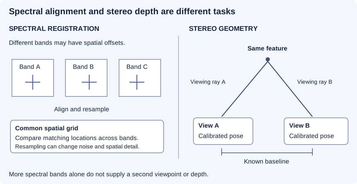
Several wavelength bands describe how a scene responds across the spectrum. Two calibrated viewpoints can provide geometric clues through the displacement of corresponding features. Aligning colour channels is not the same as reconstructing depth. A multispectral stereo system needs both reliable spectral measurements and reliable viewing geometry.
Better calibration, more informative bands and independent reference measurements may make material maps more useful. The benefit would be fewer ambiguous decisions and better-targeted follow-up work. Any claimed improvement needs to survive testing on samples or scenes kept separate from development.
Our band and mixture demonstrations are synthetic models. They illustrate why information can be gained or lost; they do not validate an unbuilt camera, identify a real mineral sample or reproduce an unavailable observation.
REPRODUCIBLE STUDY
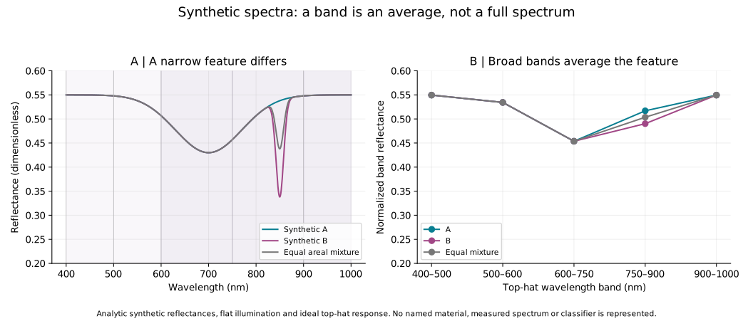
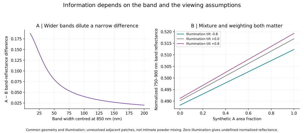
601 spectrum samples, 315 band calculations and 96 band-width cases are available. The band study includes illumination tilts of −0.8, 0 and +0.8; the interactive controls use the flat case.
A(λ) = 0.55 − 0.12 exp[−½((λ − 700)/70)²]. B(λ) = A(λ) − 0.20 exp[−½((λ − 850)/8)²], with wavelength in nm over 400–1000 nm. An areal mixture is αA + (1 − α)B.
Each ideal top-hat band reports ∫E(λ)R(λ)dλ / ∫E(λ)dλ. The controls use flat illumination. A reference measurement with the same illumination is assumed; zero denominator gives no result. The study also explores explicitly specified illumination tilts. Real filter response, atmosphere, noise and calibration error are not simulated.
These calculations show the information a chosen measurement can lose. They do not perform library classification, identify a real mineral or establish a camera's sensitivity. Spatial resolution and sampling place additional limits on every spectral image.
ANOTHER WAY TO STUDY A MIXTURE / SEPARATION OVER TIME
The very simple version: Imagine two groups going through a long hallway. One group moves ahead; the other takes longer. If they reach the door at different times, counting them separately is easier. If they arrive together, they look like one crowd.
A gas chromatograph carries a sample through a column. Different interactions with the column can make components reach the detector at different times. This is separation over time, unlike the wavelength measurements above. A small instrument could help take measurements nearer to a sample, but being small does not prove that it can separate or identify everything.
This experiment uses invented peaks. No chemical sample, real instrument, concentration or voltage is represented. We assign two equal-area Gaussian peaks and add them, to isolate the effect of spacing and width.
Try closing the gap to zero. Then keep the gap fixed and broaden the peaks. The horizontal axis is time, not wavelength.
Scroll sideways on small screens. Dotted: component A; dashed: component B; solid dark line: their sum.
| Time (s) | Component A | Component B | Sum |
|---|
Portable chemical analysis could support environmental monitoring and inspections closer to the sampling location. The useful result would be a calibrated answer about a specified substance, with known uncertainty and a checked sampling method.
A peak is not a chemical name. Different substances may have similar retention times or arrive together. Identification needs appropriate reference comparisons and, where needed, complementary detector information. Quantifying an amount requires calibration and a suitable response model.
Each curve is p(t)=exp[−(t−μ)²/(2σ²)]/(σ√(2π)). It has unit area over the full real line; its tails never terminate. The sum has area two. Our time plot shows a finite window. Unit areas are a mathematical normalization, not a claim that substances have equal detector responses.
Using extrapolated baseline tangent widths w₁=w₂=4σ, chromatographic resolution is Rₛ=2(μ₂−μ₁)/(w₁+w₂)=Δt/(4σ). A 4σ baseline width is not a full width at half maximum, which is approximately 2.355σ for a Gaussian. It also is not a sharp boundary containing the whole peak. The centres in this example are known inputs; the model does not estimate hidden components from an observed trace.
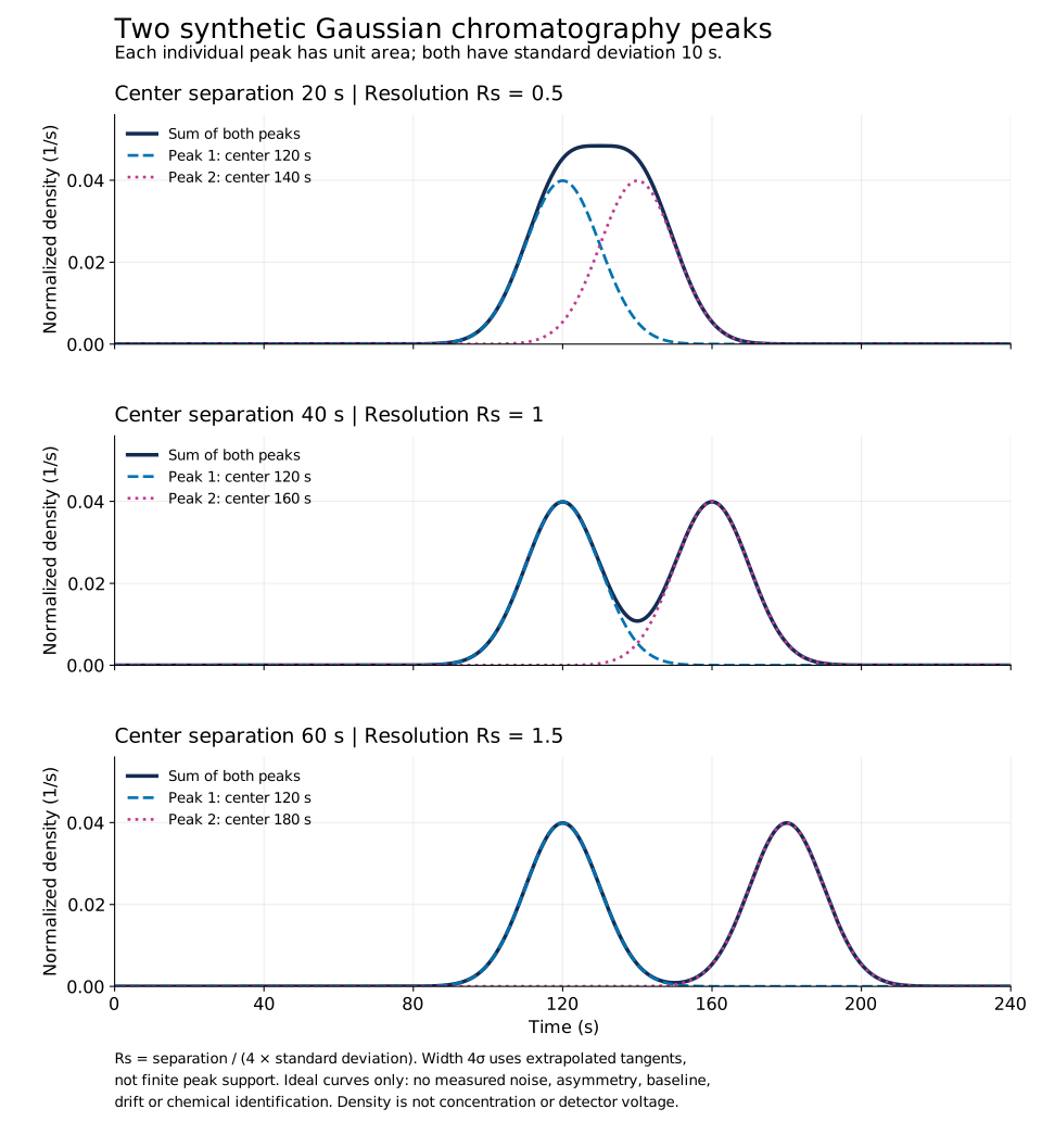
Scientific figure · PDF · Study values · CSV · Reproduce the study · Python · Methods · JSON
Missing from this model: chemical retention mechanisms, column geometry, pressure and temperature, sample injection, detector response, unequal concentrations, noise, drift and asymmetric peaks. It does not design a chromatograph, identify substances or predict miniaturized hardware performance.
What would establish a useful instrument: measurements on defined reference mixtures; retention repeatability; separation and detection limits under stated conditions; calibrated response; checks for co-eluting interferents; and comparison with a suitable reference method. A claim of miniaturization needs the actual instrument, not just a smaller diagram.
Sources: IUPAC: chromatographic resolution; IUPAC: peak-width definitions; Agilent: Fundamentals of GC, component identity, p.49; Agilent: examples of micro-GC applications. Manufacturer examples document a technology class; no product performance is assigned to our model.
Unresolved miniature-instrument proposal: this educational comparison does not recover its missing design or establish that it worked.