Imagine this
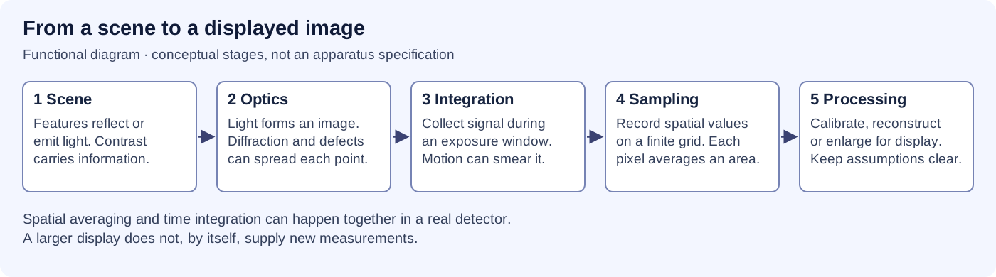
Making a picture bigger does not always show more detail. A bright spot does not prove that a place is raised. We must know what the camera measured and what a computer added.
THE FIELD GUIDE / 020 · IMAGING
Not necessarily. Every image starts with a physical measurement. An instrument records a limited signal; processing then turns it into something we can inspect. A bigger or sharper-looking display is not automatically a better observation.
Making a picture bigger does not always show more detail. A bright spot does not prove that a place is raised. We must know what the camera measured and what a computer added.
Today, knowing blur, resolution and sampling helps people choose images and avoid reading extra meaning into pixels. A distant-world reconstruction would need checks against known targets.
Computer-made examples show why a picture can be unclear; they do not prove we can recover real depth. We still need a known real object to compare with. Details filled in by software are not camera measurements.
Read-aloud starter; not yet tested with children. The fuller science, data, figures and sources follow below.
Imagine two narrow stripes. If a lens blurs them together before the sensor records them, enlarging the saved picture will not separate the original stripes. Interpolation inserts values between existing pixels. It can smooth a display without adding another observation.
Several carefully aligned images may contain extra information when their sampling positions differ. Combining them can improve a reconstruction under a tested model. A reconstructed detail can look convincing while still being wrong. Measurements, assumptions and reconstructed features must remain distinguishable.
READING A SCIENTIFIC IMAGE
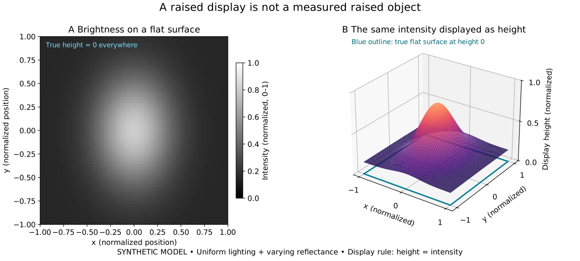
Imagine a printed label lying perfectly flat. Its centre is lighter than its edges. A computer can draw each pixel’s brightness as a height and produce an impressive hill, even though the label has no raised centre.
The figure does exactly that with a synthetic image. Nothing measured physical depth. A useful display of brightness is different from a measurement of shape.

Open the full-size two-panel figure · Open the narrow figure
| Position x | Intensity | Display height | True height |
|---|---|---|---|
| −1, left edge | 0.152244 | 0.152244 | 0 |
| 0, centre | 0.800000 | 0.800000 | 0 |
| +1, right edge | 0.152244 | 0.152244 | 0 |
Concrete use: a brightness plot can reveal uneven printing on a label. It cannot tell you that the lighter ink is physically higher. Possible next step: compare a proposed depth method on a flat patterned target and a target with independently known relief. Change the lighting and pattern to check whether the reported shape remains reliable. That comparison has not been performed here.
We assign I(x,y) = 0.15 + 0.65 exp(−[(x/0.42)² + (y/0.60)²]) on a 65 × 65 grid, with x and y from −1 to 1. True height is zero; displayed height equals I. The ideal detector is linear, lighting uniform, and reflectance varies. Shadows, perspective, blur, noise and specular reflections are omitted.
This is a counterexample to automatically reading brightness as geometry. It does not show that every method of recovering depth fails: suitable measurements, justified assumptions and independent checks can supply information absent from this display. No experimental error bars are invented.
TRY THE MODEL / SAMPLING
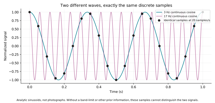
The solid and dashed lines below are synthetic brightness variations, measured relative to their mean. Black dots are ideal point samples, one unit apart. Both patterns pass through exactly the same dots. The sample list alone cannot tell which pattern produced it.
Compared frequencies: .
| Sample position | First pattern | Second pattern |
|---|
This ambiguity is called aliasing. It does not mean the object changed. To avoid it, the recorded signal must have a suitably limited range of spatial frequencies before sampling, and the sample spacing must be fine enough. This illustration uses cosine signals and ideal point samples; it does not simulate pixel-area integration, a photograph or an optical blur kernel.
TRY THE MODEL / IDEAL CAMERA
Distance spreads a small viewing angle across more ground. Aperture and wavelength set an ideal diffraction scale. Pixel size and focal length set the spacing of recorded samples. These are different quantities.
Fixed illustrative inputs: 550 nm wavelength, 5 µm pixel pitch, 2 m focal length and 4,000 pixels across. The camera looks straight down at an ideal flat plane. Rayleigh separation assumes equal incoherent point sources and an ideal circular aperture. Atmosphere, aberrations, contrast, motion and detector noise are absent from this calculation.
Ground sample distance is not a promise that every object of that size is distinguishable. A wider field of view describes coverage, not finer detail. We do not combine these outputs into a claimed real-camera resolution.
A mechanical shutter blocks light. Other optical switches redirect or modulate a beam. An electronic shutter controls when a sensor accumulates or reads charge. These mechanisms are different, even when all determine which light contributes to a frame.
Longer exposure collects more signal, but a moving image also travels farther while the frame is recorded. A faster switch cannot recover detail already lost through the optics or sampling. Trigger delay, opening and closing time, exposure duration and frame rate are different quantities. Any proposed switch needs a measured transmission change, timing and repeatability before its performance can be compared.
TRY THE MODEL / EXPOSURE
We assign a detected signal rate of 1,000 electrons per second, a background rate of 200 per second, read noise of 3 electrons RMS per exposure, and transverse motion of 0.1 metres per second at a fixed object plane. These are chosen examples, not camera specifications.
The ratio compares the expected signal with its combined noise scale. Signal and background are independent Poisson counts; read noise adds independent variance. We assume a known background mean. Saturation, dark current, changing motion and rolling-shutter distortion are omitted. Signal-to-noise and displacement are separate budgets: a moving feature may leave a detector element, so this is not a joint moving-target signal model or a recommended exposure setting.
A photoconductor becomes more electrically conductive when illuminated. In xerography, exposure changes a charge pattern on a prepared surface. Toner develops that invisible pattern into a visible one; transfer and fusing produce a durable record.
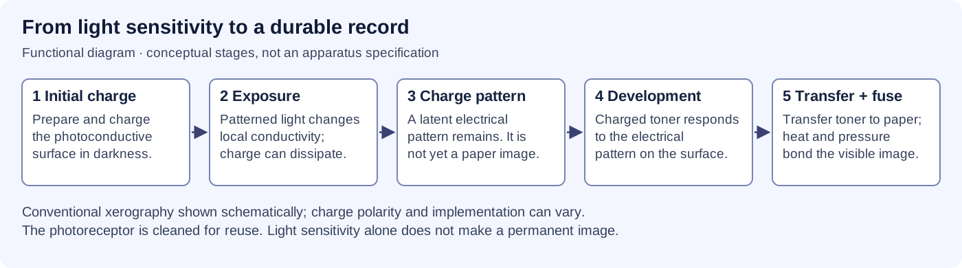
Changing conductivity alone does not explain permanent storage, readout or colour. Each step needs its own mechanism. A digital camera records and stores electronic measurements through a different chain; it is not a miniature toner copier.
An atomic-scale image is interpreted contrast from a particular instrument. It is not an ordinary photograph enlarged far enough. The interaction, detector, sample preparation and calibration determine what the image means.
| Method | What makes the signal? | What limits its interpretation? |
|---|---|---|
| Optical camera | Light reflected, transmitted or emitted by a scene | Wavelength, optics, sampling, noise and illumination |
| X-ray image | Differences in X-ray transmission through a sample | Geometry and overlapping structures; an image is not automatically a full 3D map |
| Transmission electron microscope | Electrons interacting with a prepared thin specimen | Preparation, electron optics, damage and interpretation of contrast |
| Scanning probe | A local interaction measured close to a surface | Probe shape, surface accessibility and the measured interaction |
A method that reveals atomic structure in a suitable specimen does not automatically reveal atoms deep inside any object. An instrument name alone cannot establish a new imaging capability; it needs a signal chain, reference target and independently checkable data.
A regional flood map needs different detail from a material-defect inspection. Defining the question first helps choose coverage, sampling, exposure and imaging method. A picture can be useful without showing every tiny feature.
Better detectors and calibrated combinations of multiple observations could improve useful detail. Test them on independent targets, preserve raw observations and report wrong interpretations. A sharper-looking result is only valuable if it gives a more reliable answer.
REPRODUCIBLE STUDIES
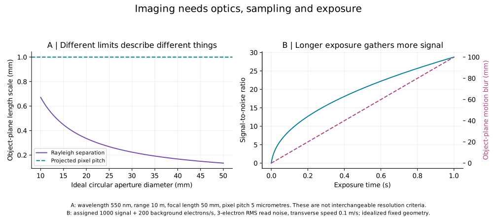
The reproducible study contains 27 camera configurations, 1,001 exposure values and 21 matching sample pairs. No measured instrument or reconstructed scene is represented.
Ideal angular Rayleigh separation is θ = 1.22λ/D; its small-angle ground projection is Hθ. Pixel spacing on the flat ground plane is Hp/f. Full field of view is 2 arctan(Np/(2f)). Here H is range, D aperture diameter, p pixel pitch, f focal length and N pixel count across.
Expected signal is S = rt and background is B = bt. SNR = S/√(S + B + σᵣ²), with zero signal giving zero SNR. Motion smear is vt in metres when v is measured in metres per second. These expected-value curves are not repeated experimental measurements and have no invented experimental error bars.
The sampling identity is cos(2πfk) = cos(2π(1 − f)k) for integer sample positions k. It establishes a specific ambiguity; it does not say every reconstruction method must fail when additional observations or justified prior information are available.
A DISTANT OBSERVATORY / SOLAR GRAVITATIONAL LENS
Gravity bends light. A proposed deep-space observatory would use the Sun’s gravity as a natural lens to study one already selected exoplanet. The lensing physics is established; sending a probe, tracking the target and reconstructing a detailed image are still mission-study challenges.
One target, one long line of travel: the spacecraft would need to travel beyond about 548 AU on the observation line for the selected star system. One parked telescope could not use the Sun as an all-sky camera for every planet.
Imagine a tiny light from a far-away planet bending around our Sun. A spacecraft would travel much farther than all the planets to catch that light. It would measure a glowing ring around the Sun, then use those measurements to try to make a map. Nobody has sent this telescope there yet.
If a future mission worked, detailed maps and spectra might help scientists compare distant planets’ surfaces, weather, oceans and atmospheres. That could improve our understanding of how planets form and which environments might be habitable. It would not by itself prove that life exists, and it offers no immediate practical service on Earth. Research value today: the studies exercise computational image reconstruction, instruments designed to block the Sun’s glare while measuring light, and navigation along a moving focal line. The methods could inform other observatories or long-range spacecraft, but that transfer and any practical benefit have not been demonstrated. See the NASA Phase II instrument and mission study, corona-aware optics analysis, and NASA Phase I navigation architecture.

Three separate questions: first, how wide is the region a spacecraft would scan? Next, how can mixed light be turned back into a pattern? Finally, how much integration does one published scenario estimate? These are separate calculations. Changing a control in one does not change the assumptions or results in the others.
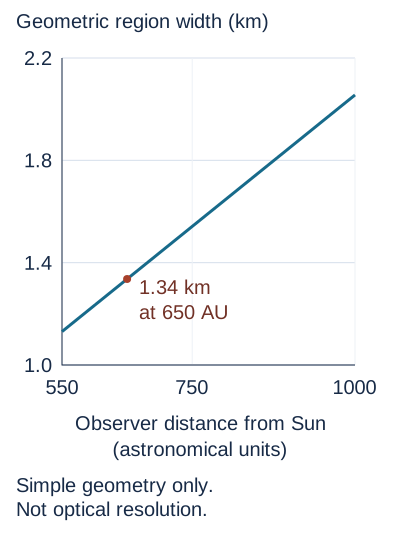
The controls change the probe’s distance and the selected target’s distance. They estimate the width of the compressed image region for a 13,000 km Earth-like planet. They do not calculate optical resolution or show a reconstructed planet.
Estimated geometric region width: 1.34 km
Focal line, not a single point. For visible light, the Phase I report derives a starting distance near 547.8 AU; the Phase II report uses about 548.7 AU. “Roughly 548 AU” is a useful rounded description. A specific mission might operate farther away to manage instrument geometry and solar-corona background; that is a mission-design choice, not a different basic lens law.
Measurements, then reconstruction. The probe would see an Einstein ring. Each part of the distant planet contributes to its brightness pattern. The telescope would scan across a very small image region and use a wave-optics model and deconvolution to estimate the source image. The Phase II report describes numerical feasibility studies; these are not photos taken by a spacecraft at the lens.
Keep lens physics separate from a reconstructed map. The Phase II report abstract quotes a maximum brightness amplification near 1011 and ideal angular resolution near 10−10 arcseconds at 1 micrometre. Neither number is the net detector signal-to-noise ratio or a demonstrated surface feature size. Its abstract describes “a few 10 km-scale” surface resolution for an Earth-like target up to 30 parsecs away. The detailed cases below have different sampling, distance, aperture and fidelity conditions, so their numbers should not be blended.
Why the published detail estimates differ. The Sun spreads the planet’s light into a ring pattern; scientists would have to measure that pattern and reconstruct a map. Here is where the often-quoted distance and resolution numbers come from. These are separate model or proposal scenarios, not observations or a matched performance comparison.
| Reported estimate | Scenario and method | Source locator and limit |
|---|---|---|
| Phase II report abstract: “a few 10 km-scale” surface resolution | Earth-like target up to 30 pc; meter-class telescope. The abstract also shows a 1024 × 1024 RGB simulation with sampled SNR near 103 per colour channel before deconvolution. The detailed conditions attached to the matching Figure 16 RGB case are listed separately below. | NASA NTRS 20250006595, report abstract / first page. The abstract does not give a complete observing recipe; do not silently apply its 30 pc reach to the detailed RGB example. |
| Phase II Figure 16: 128 × 128 monochrome; SNR about 64; under 1.5 years cumulative integration | Target at 30 pc; one-meter telescope at 650 AU. The report describes this as the top-row simulated case. | §2.4.4, printed p. 18, Figure 16 and caption, paragraphs 268–269 in the retained report text. Cumulative exposure is not a calendar schedule with travel, scanning or downtime. |
| Phase II Figure 16: 1024 × 1024 RGB; sampled SNR about 103 per colour channel and about 3 × 10³ overall; under 20 years cumulative integration | The detailed bottom-row case is a 3 pc target observed with 2.5 m telescopes at 1,000 AU. It is not the 30 pc, 100 × 100 one-year case. | §2.4.4, printed p. 18, Figure 16 caption and paragraph 270; NASA NTRS Phase II final report. Numerical illustration only; the report does not provide all scene arrays and reconstruction settings for an independent exact reproduction. |
| Phase II exposure equation: 100 × 100 samples; post-deconvolution SNR 7; about 3,000 s per sample and roughly one year total | Target at 30 pc, one-meter aperture and 650 AU observer distance. The estimate multiplies exposure per sample by 10,000 samples. | NIAC §2.4.3–2.4.4, printed pp. 15–17, paragraphs 252 and 264–265; corresponding Turyshev & Toth (2020), Eq. 153. This is an analytic exposure estimate with assumed filtering/noise conditions, not a full reproduced image or mission timeline. |
| Later Phase III proposal abstract: about 25 km surface scale after six months | Earth-like target at 30 pc; meter-class telescope beyond 547.6 AU; the abstract says this estimate includes solar-corona noise. | NASA NTRS 20205005780, attached TechPort Phase III abstract (abstract record; no verified printed-page locator). This is a later proposal summary, not a result from the Phase II final report; it supplies no matched sampling and reconstruction recipe for comparison with the rows above. |
| Landis (2017): order 200 km under a Hubble-sized imager example | A 2.4 m Hubble mirror resolving about 110 segments around a roughly 3.5-arcsecond Einstein ring; the estimate assumes a half- or crescent-phase planet and successful ring-slice deconvolution as it rotates. | NASA NTRS 20180002197, printed p. 8, §4.4. This is a distinct ring-slice approach and conditional estimate, not directly comparable to the NIAC pixel-grid examples. |
NTRS lists the Phase II report’s publication date as 18 March 2020 and its acquisition date as 27 June 2025; the latter is a catalogue date, not the report’s publication year. A source-matched comparison still needs aligned definitions of surface feature resolution, sampling, reconstruction fidelity, noise, scan coverage and exposure. Neither study nor proposal is a flight demonstration. Phase II final report record · Phase III proposal abstract · Landis study record.
Why it is hard. The planet’s light arrives close to the Sun’s much brighter apparent disk. A coronagraph or an external occulter can be studied to suppress direct photospheric light, but light from the solar corona remains a background and noise source; an instrument cannot simply remove it by blocking the disk. The target-specific optical axis also moves as the planet orbits its host star, as the host star moves relative to the Sun, and as the Sun moves relative to the Solar System barycentre. A probe would need to estimate and follow the changing image position while measuring the ring. A 2022 navigation study models these motions and discusses requirements; it is not a demonstration of spacecraft navigation at the focal line. Power, propulsion, communication over hundreds of AU, long autonomous operation and the many-year journey all remain part of an unflown architecture. Turyshev and Toth, instrument and solar-corona analysis (2022) · Turyshev and Toth, focal-line navigation analysis (2022).
Maturity records differ. The Phase II NTRS abstract assesses the studied concept at TRL 3; the NASA TechPort project record’s maturity strip reports current/end maturity 2. Both are study-stage assessments. No operational solar gravitational lens imaging mission or completed end-to-end image has been demonstrated.
Simple version: Picture a small spacecraft with a giant, light-catching sail. It first loops close around the Sun, then the sunlight pushes it far out into space. Other small spacecraft could follow like runners in a relay, passing messages and helping if one probe has trouble.
What the NASA NIAC Phase II report proposed: a possible small-satellite mission architecture for reaching the solar gravitational lens focal region and observing from there. The numbers below are study assumptions and design goals, not flight results.
On a phone, swipe sideways; with keyboard focus here, use the left and right arrow keys to read the full table.
| Mission step | Study value or concept | What it means—and what it does not |
|---|---|---|
| Small sail spacecraft | Spacecraft below 100 kg; solar sail approach spirals inward to 0.1–0.25 AU from the Sun | Proposed architecture inputs; the report does not describe a flown SGL sail vehicle. |
| Fast outward journey | 15–25 AU/year; 25 AU/year design goal; study estimates under 25 years to the focal region | Physics-based trajectory study and design goal, not a measured spacecraft speed or committed schedule. |
| Finding and staying on the right line | About 315 m/s of onboard correction Δv for a ten-year data-collection period, including barycentric motion (NASA NIAC Phase II report, paragraph 138) | The study says a future onboard propulsion system must supply this Δv budget. It is a mission requirement, not a demonstrated system capability. |
| Communications and backup | “String of pearls”: groups of small satellites launched in sequence; one example uses annual launches and ~20 AU spacing | Proposed relay, redundancy and data-management arrangement; no such deep-space relay chain has flown. |
| Power and long life | Study compares RTG-only with RTG plus radiation-hardened battery; mission analysis considers roughly 50 years | Trade study for distant, long-duration operation; it is not evidence of a built power system with that lifetime. |
Identify and characterize a suitable exoplanet before launch.
Before launchSpiral inward to 0.1–0.25 AU, then use a solar sail for the outward leg.
15–25 AU/year; 25 AU/year goalThe study baseline estimates the outward journey in under 25 years.
About 25 yearsAcquire and follow the moving focal line around 650–1,000 AU.
Up to 15 years of science operationsInside that operations window: the report separately describes an imaging phase of order 10 years as desirable. It is not an extra ten years to add after the 15-year operations allowance.
Then send the data home: at 650 AU, light alone takes about 3.75 days one way. The report does not prescribe one exact downlink calendar.
Source: NASA NIAC Phase II final report, paragraphs 35, 292, 296–297, 313 and 319–320. These are study assumptions and goals, not a funded or flown mission timeline.
This architecture makes the challenge easier to picture: there are two long journeys to solve. A probe must first travel hundreds of astronomical units, then keep finding the narrow, moving observing line while powering instruments and communicating home. The Phase II report assesses the imaging technique at TRL 3; that is an early technology-maturity assessment, not mission readiness. The authors call the concept promising and recommend further study. No operational SGL imaging mission or end-to-end flight demonstration exists.
Source: Turyshev et al., Direct Multipixel Imaging and Spectroscopy of an Exoplanet With A Solar Gravity Lens Mission, NASA NIAC Phase II report, NTRS 20250006595, mission concept section. NTRS metadata gives the publication date as 18 March 2020 and the acquisition date as 27 June 2025. The earlier Phase I study is separately catalogued as NTRS 20180006788. Phase II NASA record and report · Phase I NASA record.
For a target diameter D, observer distance z and target distance d, the simplified projected width is w ≈ D z / d. We use D = 13,000 km, d = 100 light-years, and 1 light-year = 63,241.077 AU. This reproduces the study’s approximate 1.3 km scale at 650 AU. The equation is a geometric scale estimate only; it leaves out wave optics, the telescope, pointing, noise, solar-corona background and reconstruction quality. It therefore cannot predict an actual image or decide whether the mission would work.
FROM LIGHT TO A MAP
Imagine trying to read a drawing through rippled glass. Light from one spot spreads into its neighbours. If we know how the glass spreads light, a computer can try to untangle the drawing. Small mistakes in the measurements can also grow when we do that.
The Sun’s gravitational lens has a similar challenge. The study below follows published optical equations through a small artificial example. It helps explain what image recovery does, why noise matters, and why a convincing recovered pattern still needs checking.
At a chosen wavelength of 1 micrometre and a distance of 650 AU, the spherical-Sun model spreads a point’s light into rings. Its first dark ring is about 4.91 cm from the axis in the spacecraft’s measurement plane. A 1 m telescope averages many of those rings. That centimetre value is not a claim that we could resolve centimetres on a planet.

We know the starting drawing because we made it. That lets us compare the recovered drawing with the answer. For a distant planet, we would not have that answer in advance: this exercise checks a method under chosen assumptions, not a real planetary map.
This is an artificial 6 m square in the projected measurement plane, with no light outside it. It is much smaller than the kilometre-scale region associated with a whole Earth-sized target. Each of its 24 × 24 source cells contributes light to every measurement through the aperture-averaged response. The measurement panel is a map of scan positions; it is not a photograph of the Einstein ring.

Try direct inversion with noise, then add stabilization. Stabilization reduces noise amplification but can also remove real detail. These three settings are illustrative choices, not an automatically optimized reconstruction. Think of stabilization as asking the computer to resist very large brightness values: it can tame noise but also flatten real contrast.
Panel descriptions appear here after the calculation data load. The original source contains a bright patch and narrow bar separated by a dark gap.
Measurement colours can also saturate when added noise pushes a cell outside their fixed scale. Use the numeric reader for the exact value. Rows and columns run from 0 to 23. Row 0 is the bottom of the displayed pattern. Source, recovery and error use relative brightness; measurements use the separate integrated-signal scale.
| Added noise | Stabilization | Brightness RMSE | Interpretation |
|---|---|---|---|
| None | 0 | 2.30 × 10⁻¹² | Same-model consistency check |
| 1% | 0 | 106.1175 | Noise overwhelms direct inversion |
| 1% | 0.01 | 0.1096 | Recoverable structure, remaining error |
| 1% | 0.1 | 0.1067 | More stabilization, less contrast |
The relative point response is J₀²(αρ), with α = (2π/λ)√(2rg/z) and chosen rg = 2,953.25 m. We integrate it over a 1 m circular aperture, then over each 0.25 m square source cell. The finite forward matrix includes cell area, uses zero source outside the square, and is neither wrapped periodically nor normalized row by row. Its common absolute gain is omitted; no photon rate is inferred.
Recovery minimizes ‖Ax − y‖² + γ²‖x‖². The displayed stabilization sets γ relative to the largest singular value. Run the downloadable Python script with NumPy, SciPy and Matplotlib; exact package versions are recorded in the methods file. Negative recovered values are not clipped from calculations. The noise seed is fixed at 271828 and reused between settings. Toth & Turyshev (2021), Eqs. 1 and 4–6 provide the optical forward/inverse context; this implementation and regularization experiment are independent.
The numerical aperture integral agrees with the analytic on-axis result to about 7 × 10⁻¹⁷. Doubling source-cell integration from 16 to 32 nodes per axis changes the matrix by about 1.08 × 10⁻⁷ in relative Frobenius norm. Halving radial interpolation spacing from 2 mm to 1 mm changes it by about 1.31 × 10⁻⁶. These are numerical convergence checks, not physical uncertainty bounds.
Perfect no-noise recovery is optimistic because the same model generates and reconstructs the measurements. A separate check changes the generating aperture to 1.02 m while retaining a 1 m inverse and stabilization 0.01; its no-noise RMSE is about 0.0657, versus 0.0652 without that mismatch. This tests one chosen perturbation, not general robustness.
Limits of this 24 × 24 numerical benchmark: it leaves out light from the rest of a planet, solar multipoles, changing clouds, source rotation, pointing errors, detector response, spectral bandwidth, realistic coronal noise and exposure time. Another published study below models rotation and changing illumination in a simplified simulation; those effects are still absent from this benchmark. This numerical experiment does not reproduce the NIAC report’s planet images or establish achievable planetary resolution; the separate published simulation also does not demonstrate a mission.
A published approximation considers an Earth/Sun analogue at 30 parsecs, observed from 650 AU, with reconstructed signal-to-noise ratio 7. Evaluating its exposure expression for 100 × 100 pixels and a 1 m telescope gives about 1.01 years of accumulated integration. This reproduces the arithmetic behind the roughly one-year example; it does not run that image reconstruction. It is separate from the artificial pattern above.

10,000 total pixels: calculated integration RHS 1.0114 Julian years, or 3,191.664 seconds per sample. This is the published approximation, not a mission schedule.
More pixels require both more samples and stronger measurements to retain the chosen final signal-to-noise ratio. With these inputs fixed, the calculated total grows with the square of the total pixel count. A larger aperture reduces it. For example, doubling the number of pixels along each side gives four times as many pixels and sixteen times the calculated total integration; changing a 1 m aperture to 2 m divides that total by eight, with the other assumptions fixed. Travel, manoeuvres, instrument downtime and sending data home are not included. Adding up the time spent collecting light is not the same as a mission calendar.
Eq. 153, author-manuscript page 28, writes tpixel ≤ 0.00354 N SNRR² [1 + 0.79(650/z)5.1 + 0.05(z/650)2.65] d−3(z₀/30)²(650/z)3.4 seconds, with z in AU, z₀ in parsecs and d in metres. N is the total number of pixels. We display its RHS multiplied by N for sequential integration, using 365.25 days per year.
The downloadable reproduction script accepts only the displayed fixed scenario: integer side lengths 25–200, apertures 1 or 2 m, SNR 7, observer 650 AU and target 30 pc. It rejects other inputs rather than extrapolating silently. The paper’s empirical filtering factor a = 10 and corona-dominated noise approximation are retained. They are assumptions, not proven guarantees for every scene. The selected 1 m case evaluates to 3,191.664 seconds per sample; the otherwise identical 2 m case is 398.958 seconds. These fixed-input comparisons must not be equated with separately specified megapixel illustrations.
The inspected report does not supply a complete executable reconstruction case: its exact radiance array, scan schedule and filter settings are not established here. Published derivation manuscript, Eqs. 152–153 · NIAC Phase II report, section 2.4.4.