Imagine this
A spring gives a bumpy object room to move. Another part slows the bouncing, like a bicycle shock absorber. That part is called a damper. If there is too little room, the object can still hit the end.
THE FIELD GUIDE / 001 · MECHANICS
When the world shakes, does everything have to shake with it?
A spring and a damper can give a delicate object a gentler ride. Explore how it works—and why making it softer is not always better.
Feel the difference ↗Start with the idea ↓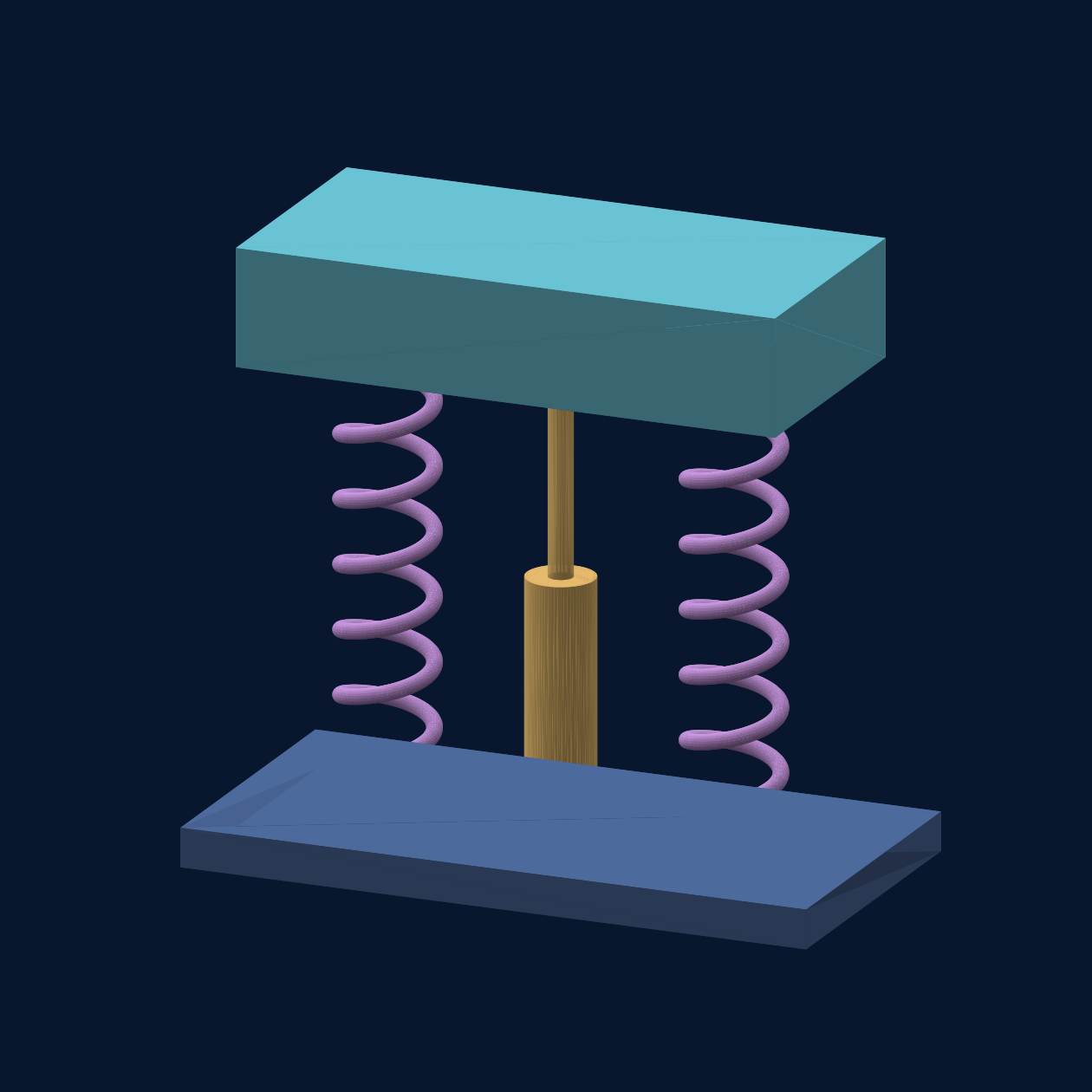
The top block is the inert mass. The two coils store energy. The central damper turns some motion into heat. All connect the mass to the moving base below.
This original conceptual CAD assembly is reduced to one ideal mass, one total stiffness and one total damping coefficient in the calculation. The springs and damper act in parallel. The lesson calculates motion in one direction only, around loaded equilibrium.
Dimensions were chosen for explanation. They do not specify the simulated mass, stiffness, damping or available travel, and do not establish a tested device or manufacturing design.
A spring gives a bumpy object room to move. Another part slows the bouncing, like a bicycle shock absorber. That part is called a damper. If there is too little room, the object can still hit the end.
Today, spring-and-damper supports reduce vibration for some instruments and equipment. This page's calculations could help choose what to test in a real mount.
A computer tried 54 chosen cases to show the trade-off. These were calculations, not real tests; friction, heat, tired parts, stops and real bumps still need checking.
Read-aloud starter; not yet tested with children. The fuller science, data, figures and sources follow below.
01 / UNDERSTAND
Imagine carrying a cup of water on a bumpy road. If you hold it rigidly, every bump reaches the cup. If your arms bend, the cup can move more gently.
An isolator does something similar. It lets a protected object move relative to its support. The challenge is giving it enough room without letting it bounce for too long.
It stores energy as it bends or stretches, then pushes the object back toward its resting position.
Like a bicycle shock absorber, it resists motion and turns some mechanical energy into heat.
A softer support often needs more travel. Run out of room and the object may hit a stop—something this simple model does not simulate.
02 / EXPERIMENT
Change the suspension. Watch the calculated motion, then compare the accelerations below.
Softer ← natural frequency → stiffer
More damping reduces bouncing, but can transmit more of a short shock.
A brief jolt and a long push behave differently.
Fixed scenario: 75 kg instrument, 1 g peak input, 25 mm available travel. These are teaching assumptions.
The drawing rescales movement to fit each scenario; compare the travel values, not the animation size. Both supports receive the same bump. The animation shows motion relative to the moving support.
Rigid mount Isolated mount
Changing the view does not change the calculation or its full-window peak values.
The table shows 100 consecutive integration samples per page. Times are seconds, acceleration is in g, and relative travel is in millimetres. The CSV contains all 8,000 samples for the current controls.
| Time (s) | Base (g) | Instrument (g) | Travel (mm) |
|---|
Time in seconds → · acceleration in g (1 g ≈ 9.81 m/s²). Curves are recalculated from the spring–damper equations, not illustrative scores.
03 / THE SURPRISE
Try “Soft & bouncy”, then lengthen the bump. The instrument can need more space and keep moving after the shock ends. Try “Stiff”: movement shrinks, but more acceleration can reach the instrument. Good design starts with the kind of disturbance you expect.
04 / WHAT THIS COULD IMPROVE
Isolate sensitive optics or laboratory instruments from floor vibration. The benefit depends on the vibration frequencies and the instrument’s tolerance.
Design protective mounts for delicate payloads. A useful next step is to measure real bumps and check the required travel.
Reduce vibration passed between a machine and its surroundings. A full design must also consider mounting geometry and multiple directions.
05 / STUDY RESULTS
What happens when we test the idea across 54 different conditions? A numerical parameter study reveals both the benefit and the space it demands.
COMPUTATIONAL STUDY · Original project calculations · Not experimental measurements or a peer-reviewed publication
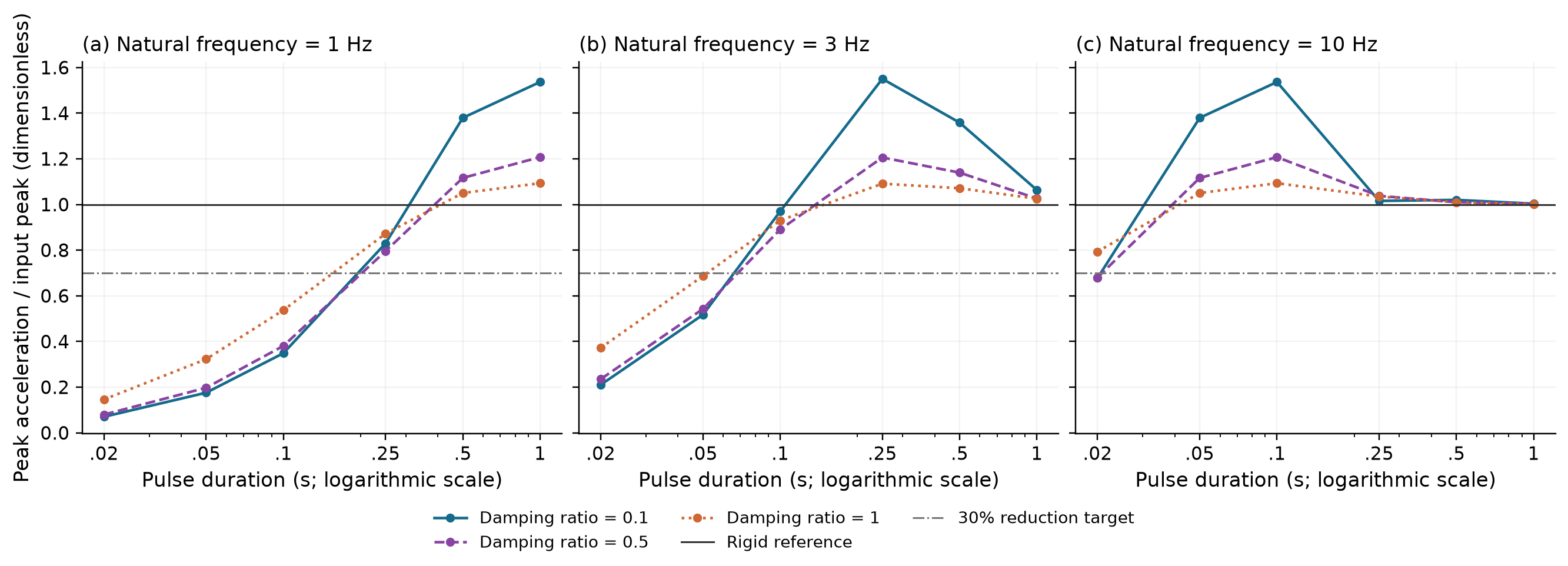
How to read it. Lower is gentler. Compare the left and right panels: a softer suspension can soften a brief jolt substantially, while a long push is harder to isolate. Some conditions amplify the peak instead of reducing it.
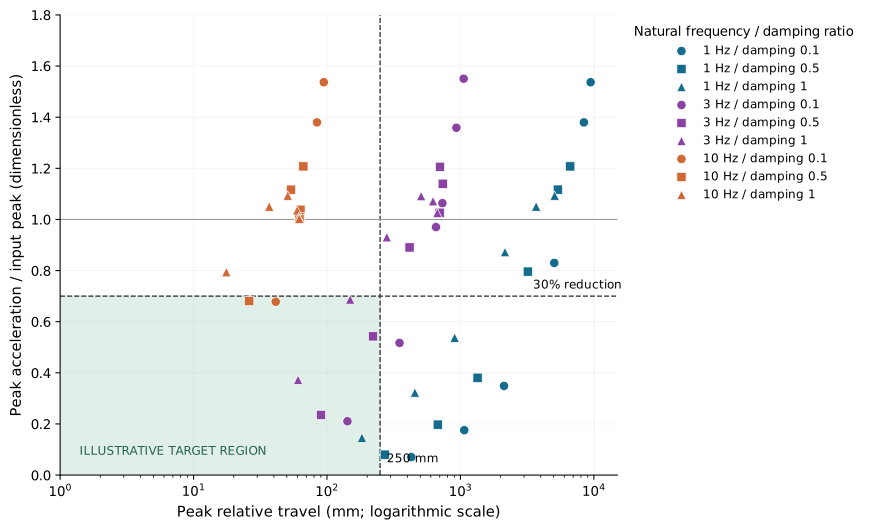
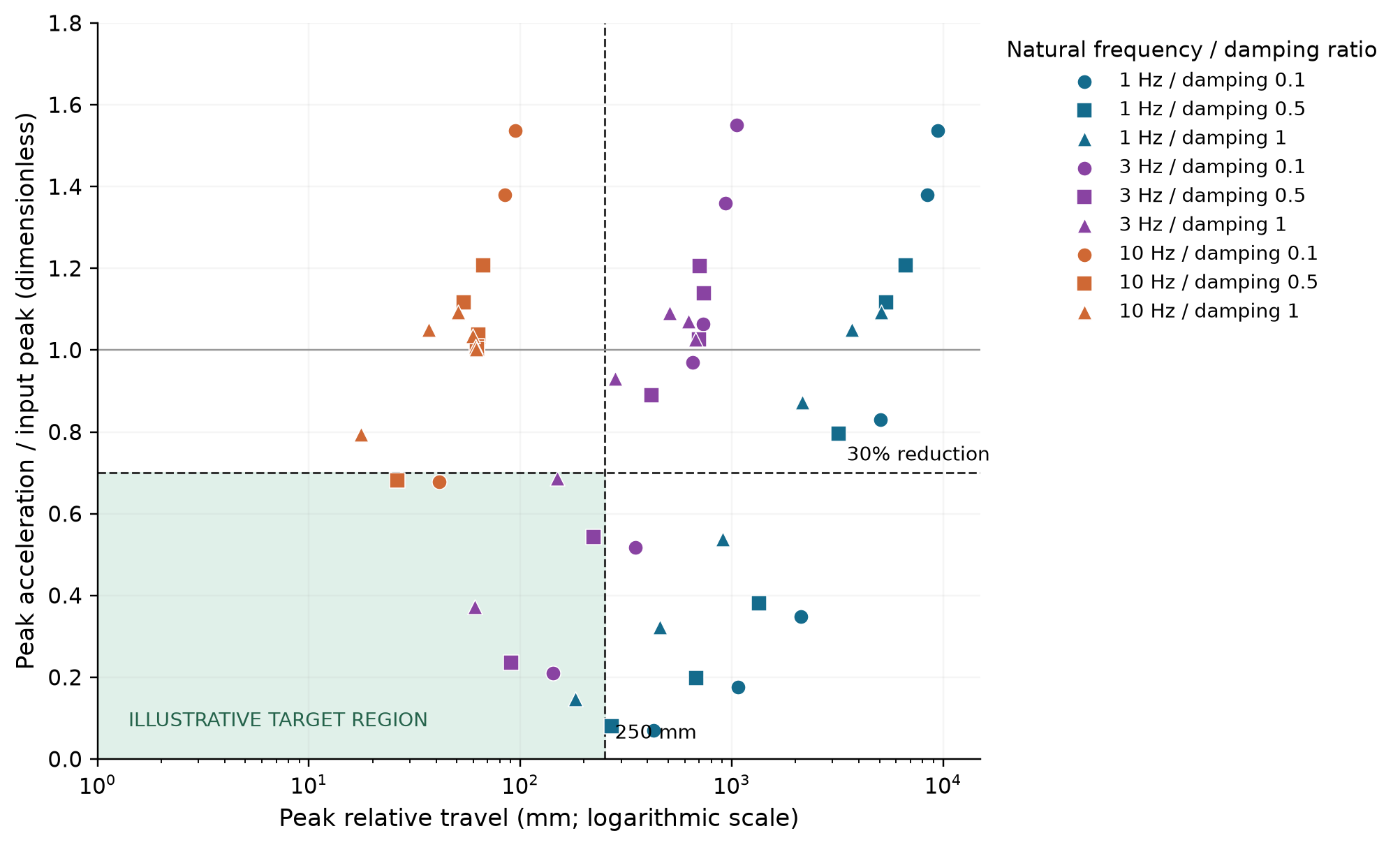
What matters. The bottom-left region is the useful compromise in this screening exercise: less acceleration, without too much movement. A very low point far to the right still needs a large mechanism. The 8/54 count describes this chosen grid; it is not a probability of success.
Archived 25 g input and 250 mm travel screen, separate from the live 1 g example. Pass requires travel strictly below 250 mm and at least 30% peak reduction. Values are rounded for display; screening uses stored unrounded values.
| Case | Pulse (s) | Frequency (Hz) | Damping ratio | Peak (g) | Travel (mm) | Reduction (%) | Screen |
|---|---|---|---|---|---|---|---|
| 1 | 0.02 | 1.0 | 0.1 | 1.760 | 428.39 | 92.96 | Outside screen |
| 2 | 0.02 | 1.0 | 0.5 | 1.995 | 271.30 | 92.02 | Outside screen |
| 3 | 0.02 | 1.0 | 1.0 | 3.652 | 182.70 | 85.39 | Pass |
| 4 | 0.02 | 3.0 | 0.1 | 5.263 | 142.37 | 78.95 | Pass |
| 5 | 0.02 | 3.0 | 0.5 | 5.884 | 90.16 | 76.47 | Pass |
| 6 | 0.02 | 3.0 | 1.0 | 9.310 | 60.72 | 62.76 | Pass |
| 7 | 0.02 | 10.0 | 0.1 | 16.954 | 41.27 | 32.19 | Pass |
| 8 | 0.02 | 10.0 | 0.5 | 17.013 | 26.14 | 31.95 | Pass |
| 9 | 0.02 | 10.0 | 1.0 | 19.845 | 17.62 | 20.62 | Outside screen |
| 10 | 0.05 | 1.0 | 0.1 | 4.390 | 1068.87 | 82.44 | Outside screen |
| 11 | 0.05 | 1.0 | 0.5 | 4.933 | 676.93 | 80.27 | Outside screen |
| 12 | 0.05 | 1.0 | 1.0 | 8.066 | 455.85 | 67.73 | Outside screen |
| 13 | 0.05 | 3.0 | 0.1 | 12.927 | 349.67 | 48.29 | Outside screen |
| 14 | 0.05 | 3.0 | 0.5 | 13.565 | 221.46 | 45.74 | Pass |
| 15 | 0.05 | 3.0 | 1.0 | 17.169 | 149.16 | 31.32 | Pass |
| 16 | 0.05 | 10.0 | 0.1 | 34.488 | 84.17 | -37.95 | Outside screen |
| 17 | 0.05 | 10.0 | 0.5 | 27.911 | 53.76 | -11.64 | Outside screen |
| 18 | 0.05 | 10.0 | 1.0 | 26.260 | 36.92 | -5.04 | Outside screen |
| 19 | 0.1 | 1.0 | 0.1 | 8.719 | 2122.78 | 65.12 | Outside screen |
| 20 | 0.1 | 1.0 | 0.5 | 9.518 | 1344.39 | 61.93 | Outside screen |
| 21 | 0.1 | 1.0 | 1.0 | 13.435 | 905.36 | 46.26 | Outside screen |
| 22 | 0.1 | 3.0 | 0.1 | 24.251 | 656.00 | 3.00 | Outside screen |
| 23 | 0.1 | 3.0 | 0.5 | 22.262 | 415.85 | 10.95 | Outside screen |
| 24 | 0.1 | 3.0 | 1.0 | 23.259 | 280.80 | 6.97 | Outside screen |
| 25 | 0.1 | 10.0 | 0.1 | 38.416 | 94.62 | -53.66 | Outside screen |
| 26 | 0.1 | 10.0 | 0.5 | 30.187 | 66.50 | -20.75 | Outside screen |
| 27 | 0.1 | 10.0 | 1.0 | 27.329 | 50.83 | -9.32 | Outside screen |
| 28 | 0.25 | 1.0 | 0.1 | 20.746 | 5050.60 | 17.02 | Outside screen |
| 29 | 0.25 | 1.0 | 0.5 | 19.898 | 3200.04 | 20.41 | Outside screen |
| 30 | 0.25 | 1.0 | 1.0 | 21.805 | 2157.82 | 12.78 | Outside screen |
| 31 | 0.25 | 3.0 | 0.1 | 38.764 | 1057.60 | -55.05 | Outside screen |
| 32 | 0.25 | 3.0 | 0.5 | 30.149 | 703.06 | -20.60 | Outside screen |
| 33 | 0.25 | 3.0 | 1.0 | 27.281 | 507.58 | -9.13 | Outside screen |
| 34 | 0.25 | 10.0 | 0.1 | 25.393 | 62.94 | -1.57 | Outside screen |
| 35 | 0.25 | 10.0 | 0.5 | 25.945 | 63.28 | -3.78 | Outside screen |
| 36 | 0.25 | 10.0 | 1.0 | 25.877 | 59.72 | -3.51 | Outside screen |
| 37 | 0.5 | 1.0 | 0.1 | 34.490 | 8417.66 | -37.96 | Outside screen |
| 38 | 0.5 | 1.0 | 0.5 | 27.913 | 5375.99 | -11.65 | Outside screen |
| 39 | 0.5 | 1.0 | 1.0 | 26.260 | 3692.48 | -5.04 | Outside screen |
| 40 | 0.5 | 3.0 | 0.1 | 33.969 | 932.62 | -35.87 | Outside screen |
| 41 | 0.5 | 3.0 | 0.5 | 28.491 | 737.21 | -13.96 | Outside screen |
| 42 | 0.5 | 3.0 | 1.0 | 26.782 | 623.32 | -7.13 | Outside screen |
| 43 | 0.5 | 10.0 | 0.1 | 25.505 | 63.32 | -2.02 | Outside screen |
| 44 | 0.5 | 10.0 | 0.5 | 25.249 | 62.41 | -1.00 | Outside screen |
| 45 | 0.5 | 10.0 | 1.0 | 25.243 | 61.49 | -0.97 | Outside screen |
| 46 | 1.0 | 1.0 | 0.1 | 38.417 | 9462.23 | -53.67 | Outside screen |
| 47 | 1.0 | 1.0 | 0.5 | 30.187 | 6650.31 | -20.75 | Outside screen |
| 48 | 1.0 | 1.0 | 1.0 | 27.329 | 5082.73 | -9.32 | Outside screen |
| 49 | 1.0 | 3.0 | 0.1 | 26.590 | 732.79 | -6.36 | Outside screen |
| 50 | 1.0 | 3.0 | 0.5 | 25.654 | 698.81 | -2.61 | Outside screen |
| 51 | 1.0 | 3.0 | 1.0 | 25.637 | 671.38 | -2.55 | Outside screen |
| 52 | 1.0 | 10.0 | 0.1 | 25.091 | 62.32 | -0.37 | Outside screen |
| 53 | 1.0 | 10.0 | 0.5 | 25.062 | 62.18 | -0.25 | Outside screen |
| 54 | 1.0 | 10.0 | 1.0 | 25.062 | 61.95 | -0.25 | Outside screen |
| Pulse (s) | Frequency (Hz) | Damping ratio | Peak (g) | Travel (mm) |
|---|---|---|---|---|
| 0.02 | 1.0 | 1.0 | 3.652 | 182.70 |
| 0.02 | 3.0 | 0.1 | 5.263 | 142.37 |
| 0.02 | 3.0 | 0.5 | 5.884 | 90.16 |
| 0.02 | 3.0 | 1.0 | 9.310 | 60.72 |
| 0.02 | 10.0 | 0.1 | 16.954 | 41.27 |
| 0.02 | 10.0 | 0.5 | 17.013 | 26.14 |
| 0.05 | 3.0 | 0.5 | 13.565 | 221.46 |
| 0.05 | 3.0 | 1.0 | 17.169 | 149.16 |
To run the independent check, place the downloaded study.json beside the reference script and run it with Python and NumPy. It compares peaks on the same 0.5 ms sample grid; it does not bound unsampled continuous-time extrema.
A 75 kg mass, supported by a linear spring and viscous damper, starts at rest. Its base receives one half-sine acceleration pulse with a 25 g peak. We combine 3 natural frequencies (1, 3, 10 Hz), 3 damping ratios (0.1, 0.5, 1) and 6 pulse durations (0.02–1 s).
The equations are integrated for 4 s with fourth-order Runge–Kutta and a 0.0005 s time step. These figures report calculated maxima within that window. There are no statistical error bars because these are deterministic runs, not repeated measurements.
The calculation demonstrates a trade-off within an idealised one-dimensional model. The 250 mm travel and 30% reduction thresholds are illustrative screening choices, not validated engineering requirements.
Travel stops, friction, nonlinear springs and heat are omitted. A numerical sensitivity check halved the time step: peak acceleration changed by at most 0.003864 g and travel by 5.476 micrometres across the 54 cases. Extending the simulation from 4 to 15 seconds changed neither maximum. All screening classifications stayed the same. An independent closed-form solution was also compared at the same sample times: the largest peak-acceleration discrepancy was 0.000000544 g, with all classifications unchanged. These checks validate the numerical solution of the assumed equations, not their fit to a real device. Physical model validation remains necessary. The interactive experiment above uses a milder 1 g input and a 25 mm travel allowance; these plots retain the recorded study’s original conditions.
A HYPOTHETICAL DESIGN QUESTION
Imagine a 75 kg instrument with 25 mm of allowed relative movement about its equilibrium position. Assign a 1 g half-sine bump lasting 0.05 seconds. Choose a natural frequency of 3 Hz and damping ratio 0.5.
The model gives a sampled peak of 0.543 g and 8.86 mm of relative travel: a 45.7% peak reduction. Against hypothetical goals of at least 30% reduction and no more than 25 mm of relative travel, this case passes both numerical checks. These goals are teaching choices, not an instrument's certified limits.
The effective total stiffness would be about 26.6 kN/m and viscous damping 1.41 kN·s/m, from k = m(2πf)² and c = 2mζ(2πf). They describe the complete ideal support, not each individual mount or an available product.
Dynamic travel is not total device size. Springs, damper stroke, attachments, stops, tolerances and clearance require additional space. If this same ideal spring carries the weight vertically, static compression is about 27.6 mm before the bump. The 8.86 mm response is measured around that loaded equilibrium. Preload and support geometry need their own account.
These are maxima over the existing 0.5 ms sample grid, not bounds on every instant. The model omits friction, stops and nonlinear effects. It does not establish hardware safety, a purchasing specification or a cost saving.
This is a measurement-evidence plan, not a construction guide or shock-test operating procedure. No physical test was performed for this page.
06 / WHAT WE ACTUALLY KNOW
Spring–damper isolation is conventional mechanics. This chapter offers a numerical experiment, not a new material or a tested product.
The project contains a 54-case numerical study. Under its original 25 g shock assumptions, 8 cases met both illustrative screening rules: at least 30% lower peak acceleration and less than 250 mm travel. Those rules are not safety limits.
Real springs and dampers are not perfectly linear. Hardware tests must establish friction, heating, fatigue, mounting behaviour and what happens at a travel stop.
Relative displacement x obeys:
x″ + 2ζω x′ + ω²x = −abase(t)ω = 2πf; f is natural frequency, ζ is damping ratio. The input is a half-sine acceleration pulse. Instrument acceleration is −2ζωx′ − ω²x.
The simulator uses fourth-order Runge–Kutta, a 0.0005 s step and a 4 s window. It starts at rest and omits stops, nonlinear effects and additional degrees of freedom. The live model uses 1 g; the recorded study used 25 g.
Download the 54-case study (JSON) ↗READ FURTHER
These sources explain the underlying methods and real applications. They do not validate the particular simulations on this page.
A teaching lecture on springs, damping and how vibration passes from a source to a receiver. Its discussion of sustained vibration complements our single-shock experiment.
A published research record describing a spring-and-viscous-damping system with six degrees of freedom. This is a more complete physical system than our one-dimensional idealisation.
Hertz (Hz): cycles per second. Natural frequency: the rate at which an ideal undamped system oscillates after a disturbance. Damping ratio: a measure of resistance to oscillation; a ratio of 1 is critical damping in this linear model. Resonance: a strong response when repeated excitation interacts with the system’s natural motion.
Chapter revised 27 September 2026. Original site figures are numerical results; linked literature retains its own authorship and rights.