Imagine this
If you know where landmarks are, measure which way they are. Where the direction lines meet can show where you are. Slightly wrong readings or poor angles make the answer uncertain.
THE FIELD GUIDE / 002 · NAVIGATION
Knowing which way to look is not the same as knowing where you are.
Imagine standing on a plain with a compass and a map. Two familiar towers give you two directions. Where those lines cross is your estimated position. A tiny angle error moves the crossing—and the arrangement of the towers determines how far.
Move the landmarks ↓If you know where landmarks are, measure which way they are. Where the direction lines meet can show where you are. Slightly wrong readings or poor angles make the answer uncertain.
Bearing geometry explains how landmarks can locate a receiver and which directions are useful. A positioning system needs real sensor and map tests.
The page uses chosen layouts and synthetic noise and assumes landmark positions are known; it does not validate a deployed location system.
Read-aloud starter; not yet tested with children. The fuller science, data, figures and sources follow below.
01 / EXPERIMENT
Four known landmarks surround part of your horizon. Change their angular spread to see how geometry changes the error. Each dot is a position estimate from a fresh set of noisy angle measurements.
The angle from the first to the last landmark.
Standard deviation of independent Gaussian errors. Zero means perfect measurements.
All four landmarks stay equally far from the observer.
200 synthetic trials. Sliders reuse the same seeded random draws, so changes are easier to compare.
| Trial | x (m) | y (m) | Error (m) |
|---|
02 / UNDERSTAND
When sight lines almost overlap, you can move a long way along them without changing their angles very much. Spread the landmarks across your view and movement becomes easier to detect.
More landmarks do not automatically solve a poor arrangement. What matters is whether they provide different information.
This model treats every landmark coordinate as exact. A bad map creates another source of error.
An angle tells you a line, not a distance. Here every angle shares a perfectly known compass orientation.
Noisy lines rarely meet at one point. The model finds the position with the smallest sum of squared perpendicular distances to the lines.
03 / STUDY RESULTS
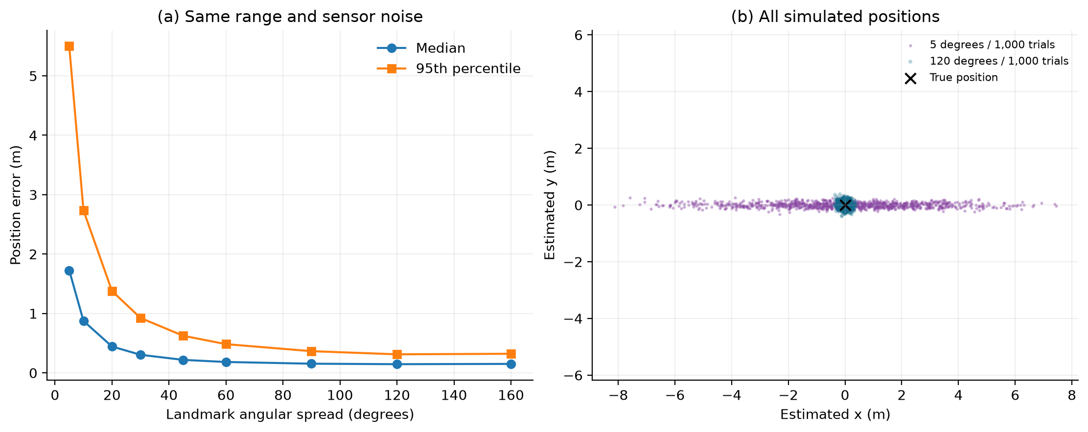
To isolate geometry, we held distance and sensor noise constant: four landmarks at 100 m, with 0.1° angular standard deviation.
COMPUTATIONAL STUDY · Synthetic measurements · Not an experimental or peer-reviewed result
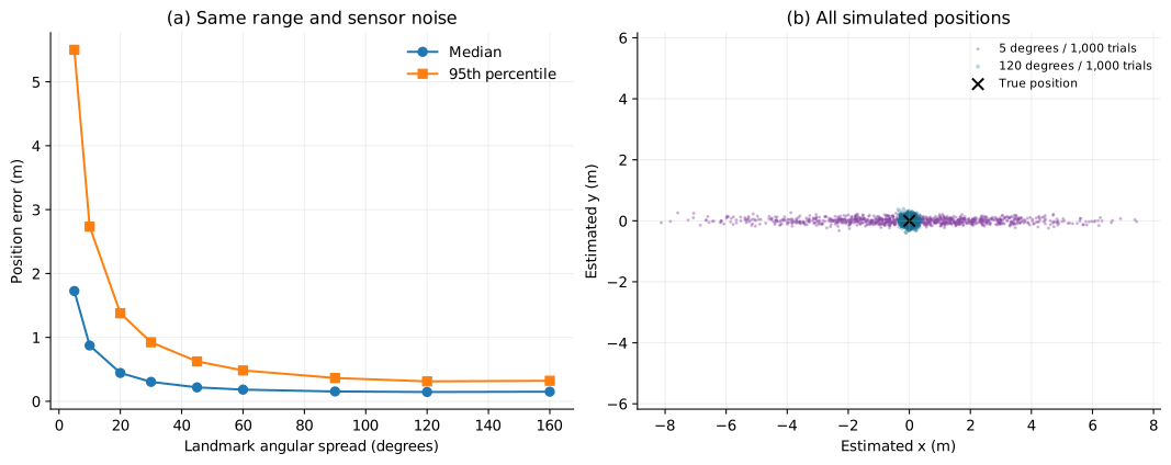
Read it simply. At 5° spread, half the errors are below 1.726 m. At 160°, half are below 0.151 m. In this controlled example, changing the arrangement helps even though the sensor stays the same. It is not a universal improvement factor for real navigation.
| Spread (degrees) | Median error (m) | 95th percentile (m) |
|---|---|---|
| 5 | 1.726 | 5.502 |
| 10 | 0.874 | 2.734 |
| 20 | 0.444 | 1.378 |
| 30 | 0.305 | 0.924 |
| 45 | 0.219 | 0.624 |
| 60 | 0.183 | 0.484 |
| 90 | 0.154 | 0.365 |
| 120 | 0.146 | 0.312 |
| 160 | 0.151 | 0.322 |
Four landmarks are equally spaced in angle, all 100 m from the true observer at (0, 0). For each trial, independent Gaussian errors with 0.1° standard deviation are added to their bearings. A least-squares line intersection estimates position. The study uses 1,000 trials per setting and seed 27092026.
The widget uses the same estimator with 200 trials and a different random generator. Its sample statistics need not equal the stored 2D study. Numerical checks recover the exact position without noise, reject exactly aligned noise-free geometry and confirm that doubling all ranges doubles the errors.
The landmark map and orientation are exact. There are no shared compass biases, hidden landmarks, wrong identifications or map errors. The estimator fits infinite lines; it does not enforce forward-facing rays and is not generally the maximum-likelihood estimator for angular noise.
A noisy, truly aligned configuration can still produce numerical answers. That does not make the geometry identifiable: set both spread and noise to zero to expose the ambiguity. A real system needs uncertainty analysis and measurements against independently known positions.
For each measured bearing θ, use the unit normal n = (−sin θ, cos θ). With landmark position s, form A = Σnnᵀ and b = Σnnᵀs. Solve Ax = b. The squared distance error is ‖x − xtrue‖². Numerically singular systems are rejected.
04 / WHAT THIS COULD IMPROVE
When planning a route, ask whether the robot sees landmarks from useful directions, not just how many it sees.
The same geometry explains why repeating almost the same view can add less information than a well-chosen new one.
Explore placement before specifying a more expensive sensor. This model illustrates the trade-off; it does not estimate costs or guarantee performance.
READ FURTHER
The mathematical foundation for fitting inconsistent measurements with a least-squares solution. The navigation model here is our own application of that method.
Why uncertainty analysis must account for more than random noise. Our simulation omits map errors and common orientation bias; the plotted percentiles should not be treated as a complete real-world uncertainty budget.
These references support the methods, not experimental validation of this teaching model. Reviewed 27 September 2026.
Use the default setting: four landmarks are each 100 metres from the true observer, at directions −45°, −15°, +15° and +45° in the same map reference. Their total spread is 90°. We assume that the map coordinates and the observer's heading are known exactly. Each measured direction receives independent Gaussian noise with a standard deviation of 0.1°.
In the stored 2D study, the 90° setting gives a median position error of about 0.154 metres and a 95th-percentile error of about 0.365 metres over 1,000 generated trials. These describe simulated errors under the stated assumptions. They are not a compass specification or a confidence interval. The live demonstration uses 200 trials and a different random generator, so its displayed summaries need not equal these values.
Here the landmarks are known and the observer's position is unknown. To locate a transmitter from bearings taken at known receiver positions, the known and unknown roles are reversed. The measurements still need positions, directions and a common reference frame.
A recording that lasts several minutes supplies a duration, not a bearing, distance or position. Travel-time ranging would require a defined emission and reception timing model, a propagation speed and a treatment of clock offsets; the duration of a recorded message alone supplies none of those. Finding a direction also does not identify the source's physical origin. Missing measurements cannot be reconstructed from a precise-looking time label.
| Displayed 2D teaching study | Separate 3D benchmark |
|---|---|
| Four landmarks at a common 100 m distance; angular spread changes. Noise is 0.1° in the plane. Nine settings, each with 1,000 trials. | Four synthetic landmarks in three spatial arrangements. Their distances differ between arrangements and are expressed in parsecs. There are 1,000 trials per arrangement. |
| Two position coordinates, with exact map and known heading. These calculations supply this page's scientific figures. | Three position coordinates in a known Cartesian frame. Noise is 1 arcsecond per tangent-plane component, not 1 arcsecond radial RMS. |
| Holding distance fixed helps isolate the effect of the chosen angular spread within this model. | Both geometry and distance vary. A difference in error cannot be attributed entirely to angular arrangement. |
The older 3D benchmark is not the data behind the figures on this page. In its noisy aligned case, the solver returns positions even though the corresponding exact geometry cannot uniquely determine position. A numerical answer is not proof that the available measurements identify the unknown.
The download contains 9,000 calculated positions: 1,000 trials for each of nine angular spreads. The same trial ID uses the same four noise draws across settings. These are paired comparisons, not 9,000 independent noise vectors. No trial fails in these nine stored settings.
All 9,000 trials · CSV · Nine summaries · CSV · Reproduce the trial export · Reference results · Methods · Validation
The current simulator export is separate. It includes settings, seed, total attempts and failed count, followed by solved estimates. Its solved index numbers the retained estimates, not the original attempt: individual failed attempts are not retained. A metadata row is included even when every attempt is singular.