Imagine this
A planet’s mass tells how much stuff it has. Its size tells how much room that stuff takes up. Average density means how tightly the stuff is packed across the whole planet.
THE FIELD GUIDE / 035 · PLANETARY PHYSICS
A planet's mass and size tell us its average density and, under a spherical approximation, its surface gravity. They do not reveal a complete map of the interior.
Change mass and radius ↓A planet’s mass tells how much stuff it has. Its size tells how much room that stuff takes up. Average density means how tightly the stuff is packed across the whole planet.
Mass and radius observations help scientists compare planets and test simple interior models. More observations may narrow the possibilities.
Average density and layered examples do not uniquely reveal interior composition.
Read-aloud starter; not yet tested with children. The fuller science, data, figures and sources follow below.
A planet crossing its star can reduce the light reaching a telescope. The transit helps constrain the planet's size relative to the star. The planet's gravitational pull can also affect the star's measured motion. Interpreting these signals requires a model: stellar properties, viewing geometry and uncertainties matter.
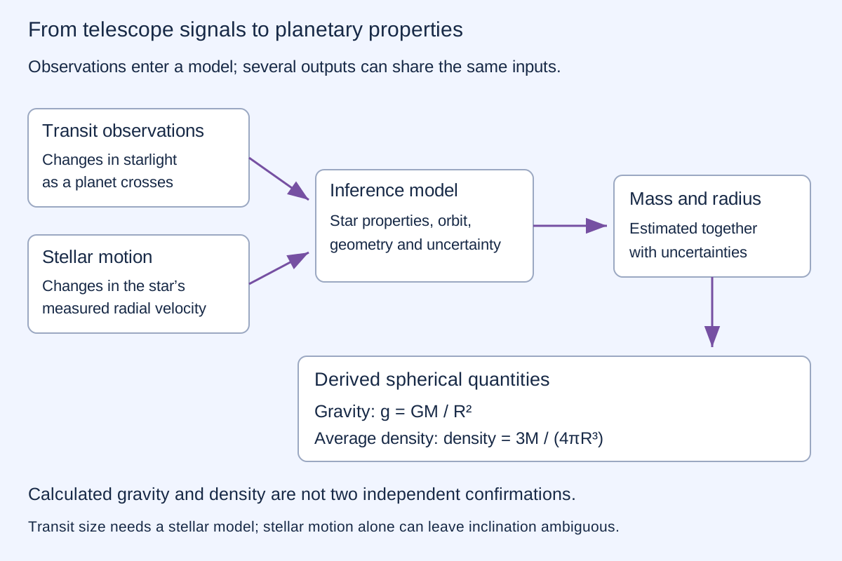
Mass, radius and gravity printed in a table may not be three independent measurements. If gravity was calculated from mass and radius, their agreement is expected. It is useful for finding arithmetic mistakes, but does not independently establish a planet's existence or identity.
NASA explains the distinct observation methods. Matching a few broad properties is not enough to identify a particular planetary system.
Before combining star-catalogue estimates, check that they refer to the same object, coordinate frame and observation epoch—the date to which the coordinates apply. A star's apparent position can change with motion and viewpoint. Two numbers can disagree because they describe different things, not simply because one instrument is less precise.
A weighted average gives some estimates more influence than others. Suppose two catalogues copied the same original measurement: counting them twice does not add an independent observation. Weights need a stated basis, and shared errors must be considered. Averaging cannot repair a common calibration error or settle which star was observed. A proposed catalogue combination without its input values, weights and uncertainty relationships cannot be reproduced or judged optimal.
HYPOTHETICAL SPHERE · NOT AN OBSERVED PLANET
Choose the mass and radius of a spherical, non-rotating model. The starting values are rounded teaching inputs. No value in these controls is a new telescope measurement.
Mean density in SI units: . Divide kg/m³ by 1000 to obtain g/cm³. Displayed digits help compare calculations; they do not create measurement precision.
Keep mass fixed and double radius: gravity falls to one quarter and average density to one eighth. Radius matters more strongly in density because a sphere's volume grows as its radius cubed. Some slider combinations need unrealistically dense or diffuse material; this lab checks arithmetic, not planetary stability.
For mass M in kilograms and radius R in metres: g=GM/R² and ρ=3M/(4πR³). We use G=6.67430×10⁻¹¹ m³ kg−1 s−2. Real orbital measurements often constrain GM directly; this lab instead assigns mass and holds G fixed.
For small, independent input standard uncertainties, u(g)/g≈√[(u(M)/M)²+4(u(R)/R)²] and u(ρ)/ρ≈√[(u(M)/M)²+9(u(R)/R)²]. These are first-order approximations. The higher settings make this approximation less exact; zero means zero assigned contribution, not perfect real knowledge.
Mass and radius estimates can share errors. A covariance term would then be needed. Their derived gravity and density are also correlated, so the two outputs are not independent confirmations. G itself has uncertainty, which is omitted here explicitly. A standard uncertainty is not a guaranteed bound or automatically a 95% confidence interval.
Rotation and shape are omitted. At the equator of a rotating spherical approximation, effective gravity includes a subtraction ω²R, where ω=2π/rotation period. Real rapid rotation also changes the shape and gravity field; this expression alone cannot predict breakup. An ellipsoid's volume is 4πa²c/3, not the volume of a sphere with an arbitrarily selected radius.
Imagine two models with identical outside radius and mass. One has a small dense core; the other has a larger, less dense core. If the surrounding region is chosen appropriately, both give the same average density.
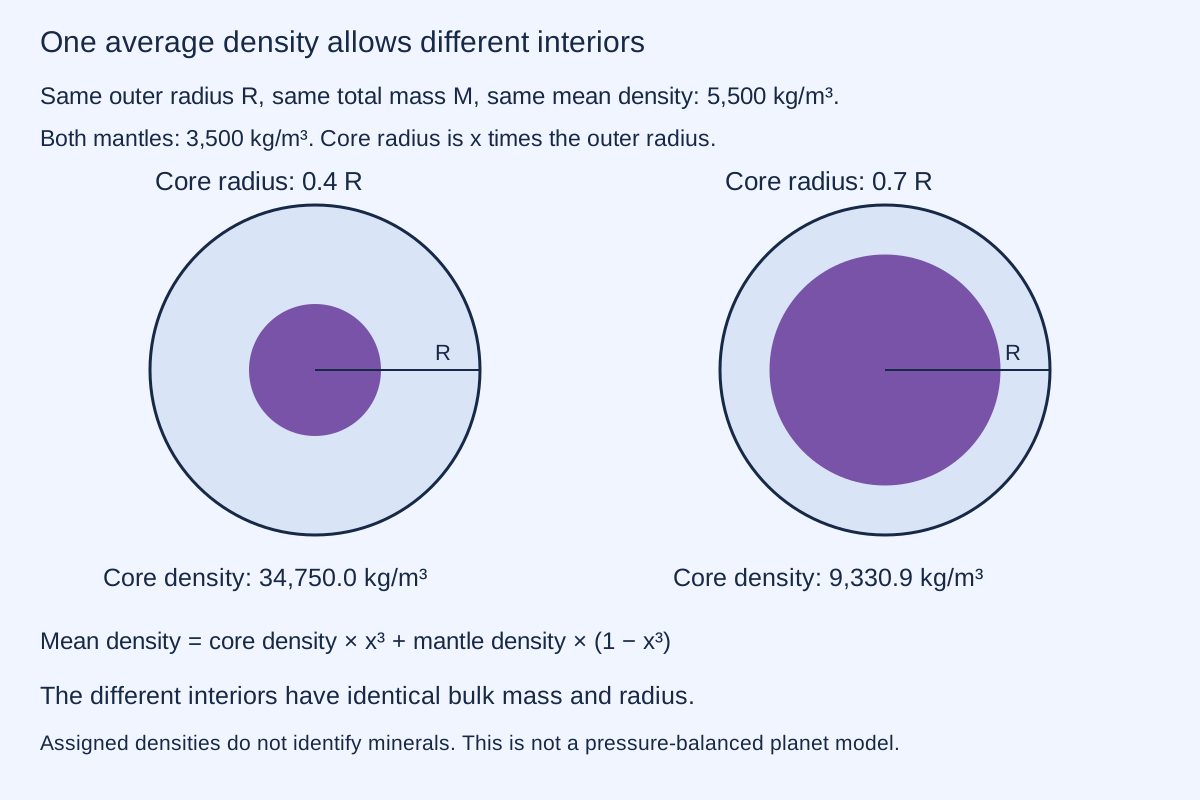
TWO CONSTANT-DENSITY REGIONS · NO PRESSURE MODEL
This separate example fixes mean density at 5500 kg/m³ and keeps the same outside radius for every comparison. It is not linked to the mass/radius controls above. Choose a core size and an outer-region density; calculate the core density needed to preserve total mass.
Let x be core radius divided by outside radius. Its fraction of volume is x³. Then mean density is ρ̄=ρc x³+ρm(1−x³). For chosen outer-region density ρm, solve ρc=[ρ̄−ρm(1−x³)]/x³. All controls keep densities positive and the core at least as dense as the outer region.
The range 0.2–0.8 excludes the degenerate endpoints: at zero core radius no core density can be inferred, while at unit core radius there is no outer region to infer. A large density at a small core radius is a mathematical solution, not evidence that a material can sustain it.
The normalized moment of inertia describes how far mass lies from the rotation axis. For these concentric constant-density regions, C/(MR²)=(2/5)[ρc x⁵+ρm(1−x⁵)]/ρ̄. A uniform-density sphere gives 0.4. Changing the mass distribution changes this extra quantity while mass and outside radius stay fixed.
No pressure balance, temperature, equation of state, phase change or formation history is modelled. The drawing cannot establish real core boundaries, a mineral composition or hidden gas reservoirs. Even an additional moment-of-inertia estimate would constrain possibilities rather than automatically identify a unique composition.
Gravity variations, rotational behaviour and, where measurements are available, seismic waves can probe different aspects of an interior. Each introduces its own model and uncertainties. A detailed drawing of many layers remains a proposed explanation unless observations constrain those boundaries.
Today: these checks help catch unit or transcription errors, interpret mass-radius diagrams and distinguish independent observations from derived numbers.
A possible next step: compare several material and thermal models with additional observations to narrow the possibilities. Mean density alone does not establish habitability, mineral deposits or usable engineering resources.
DETERMINISTIC CALCULATIONS · ASSIGNED UNCERTAINTIES
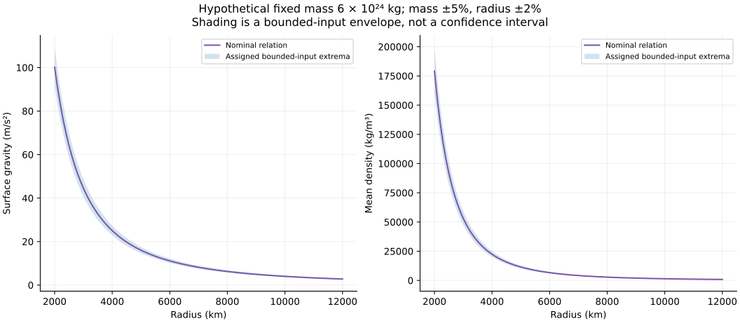
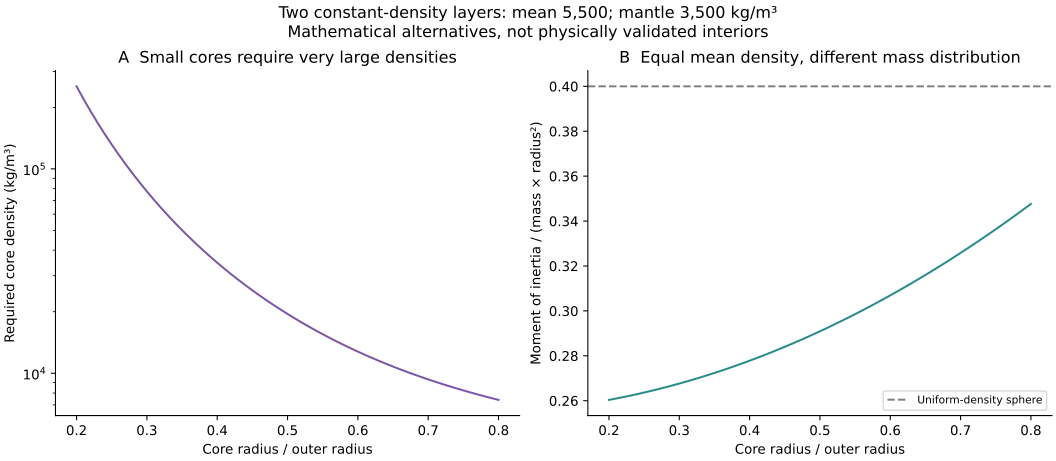
603 calculation rows: 441 mass/radius combinations, 101 radius-and-uncertainty points, 61 interior alternatives. Inputs are assigned; no measured error bars or new observations are claimed.
Run the standalone script with Python, NumPy and Matplotlib. Runtime and generator SHA-256 are recorded. With positive bounded inputs, minimum gravity and density use the smallest mass and largest radius; maxima use the largest mass and smallest radius. Unlike a propagated standard uncertainty, these extrema follow from declared hard bounds.
Scaling and units are checked independently. Finite-difference derivatives are compared with the uncertainty formulas, and integrated layer masses and shell moments with the closed-form interior expressions. These checks establish agreement within the declared mathematical models, not the existence or composition of a planet.
NASA/JPL constants · NASA observation methods · NASA-hosted review: The Inner Solar System's Habitability Through Time
The review provides context on composition and interior evolution; it is not a derivation or validation of this two-region illustration. Historical calculations remain separate. The public examples use neutral hypothetical inputs and make no discovery or identification claim.