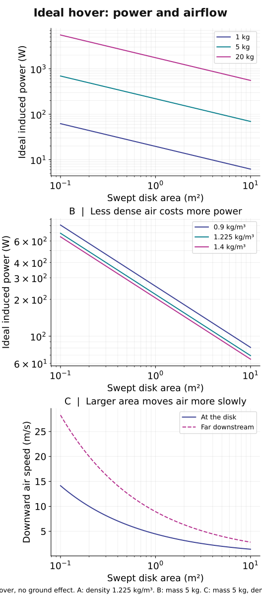
Imagine this
A strong wind can push a kite. If we take energy from moving air, that air slows down. An engine would need to count everything it loses and gains.
THE FIELD GUIDE / 010 · MOMENTUM & POWER
Explore a hypersonic concept and a heat-recovery path, then compare hovering, exhaust and magnetic forces. Every design needs an energy source and a complete momentum balance.
Draw a boundary around the machine. What crosses it? What lies outside it? These questions distinguish a force on one component from a force on the whole machine.
Explore the propulsion designs ↓A CLEARER ROUTE THROUGH THE CHAPTER
This chapter brings several kinds of propulsion together. Start with the simple explanation, then jump to designs, energy recovery, flight evidence or existing spacecraft engines. Every block can be read on its own.
A strong wind can push a kite. If we take energy from moving air, that air slows down. An engine would need to count everything it loses and gains.
Today, hot-flow, engine and electric-thruster research can improve measurements and models. A future hypersonic loop might move energy within an engine, but a vehicle benefit is still unproven.
Separate calculations and a ground-tested hot-gas generator component exist. No cited result demonstrates net vehicle energy savings or extra thrust for the complete inlet-to-accelerator loop.
Read-aloud starter; not yet tested with children. The fuller science, data, figures and sources follow below.
THE SIMPLE VERSION · NO BACKGROUND NEEDED
Imagine a very fast stream of air entering an engine. The inlet’s shape and pressure slow the air; some of its motion energy becomes pressure and heat carried by the air. No new energy appears.
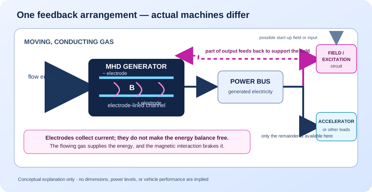
One research idea is to pass some of this hot gas through a magnetic field. When gas that can carry electricity moves through the field, a voltage can form across it and drive current through electrodes—conductive surfaces touching the gas. Taking energy this way pushes back on the moving gas and slows it. The costs depend on how the gas is made conductive and how the magnetic field is produced. Count start-up energy and any continuing power demand separately. Wires could route part of the output to another section that pushes exhaust backwards. Pushing air backwards can push a vehicle forwards, like swimming by pushing water behind you.
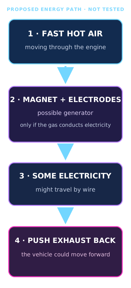
If a complete design worked, it might let an engine move some energy from one part of the flow to another. That could be useful at very high speeds. But a drawing or calculation cannot show that the whole engine would save fuel, make more useful thrust or be safe.
What has been shown: researchers have analyzed bypass-cycle models, and a separate ground-tested generator component produced electrical power from hot scramjet exhaust. What has not been shown: a complete hypersonic engine with this inlet-to-accelerator loop delivering a net vehicle benefit. Compare the studies ↓
515.7 kJ/kg is not a bucket of spare electricity. In the ideal inlet example below, it measures how much moving energy per kilogram becomes energy carried in the slower, hotter air. If 1 kg of air passed each second, that would correspond to 515.7 kW of flow-energy change before conversion—not 515.7 kW of electricity the engine could collect. The inlet calculation has no generator or electricity collection in it. An MHD generator also takes energy from the moving gas and pushes back on it; the gas must lose electrical and other losses before any output could reach an accelerator. The costs depend on how the gas is made conductive and how the magnetic field is produced. Count start-up energy and any continuing power demand separately.
Under the stated ideal-gas assumptions, the exact kinetic-energy change is 3,094,399/6 joules per kilogram. In base 12, that same value is 20A559.2₁₂ J/kg, where A means ten. The rounded 516 kJ/kg is 370₁₂ kJ/kg. One sixth ends neatly in base 12 because twelve is divisible by three; this is a convenient notation for this fraction, not extra physical precision.
The base-12 and decimal checks agree on the underlying result. Changing the number system cannot reduce measurement uncertainty or turn this ideal change in the air’s motion and heat into measured electrical output. The site keeps SI quantities in the standard decimal form used by the source literature.
See where the 515.7 kJ/kg comes from ↓ Compare it with the separate electricity model ↓
For the full scientific layer, continue to the design studies, equations, interactive ledgers, sources and limitations below. The simple explanation and the technical analysis follow the same evidence.
DESIGN ATLAS / FORM FOLLOWS THE JOB
Hypersonic atmospheric flight, stationary observation and gradual orbital travel impose different demands. Start with the job, then choose the layout. These original concept studies explain the choices; they are not optimized vehicles or manufacturing plans.
Near term, careful hypersonic research can improve measurements, heat-resistant materials, inlet and engine models, and the ability to test high-speed flows. Those tools can strengthen aerospace knowledge and related high-temperature engineering. A future transport use is only a possibility: it would require safe, reliable, affordable vehicles and demonstrated environmental and community benefits. Today’s concept drawing and separate component tests do not establish those outcomes.
NASA’s uncrewed X-43A research flights showed that a scramjet could operate for a short time in flight at hypersonic speed, producing valuable data. The aircraft was a research experiment carried by a booster—not a passenger vehicle, and not a test of the MHD bypass loop discussed here. NASA X-43A mission record.
PRIORITY / HYPERSONIC ATMOSPHERIC FLIGHT
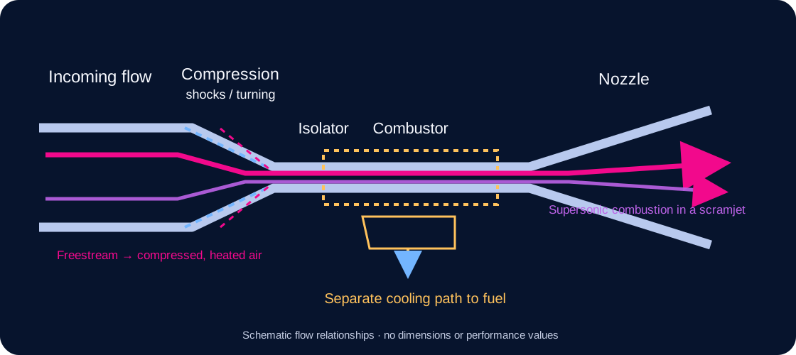
Design brief: a conceptual air-breathing research vehicle for hypersonic cruise. Hypersonic flight generally means above Mach 5—five times the local speed of sound. The model shows an editable, parametric CAD cutaway of an integrated air-breathing flowpath. It is not a complete or dimensioned aircraft design. NASA's hypersonics overview.
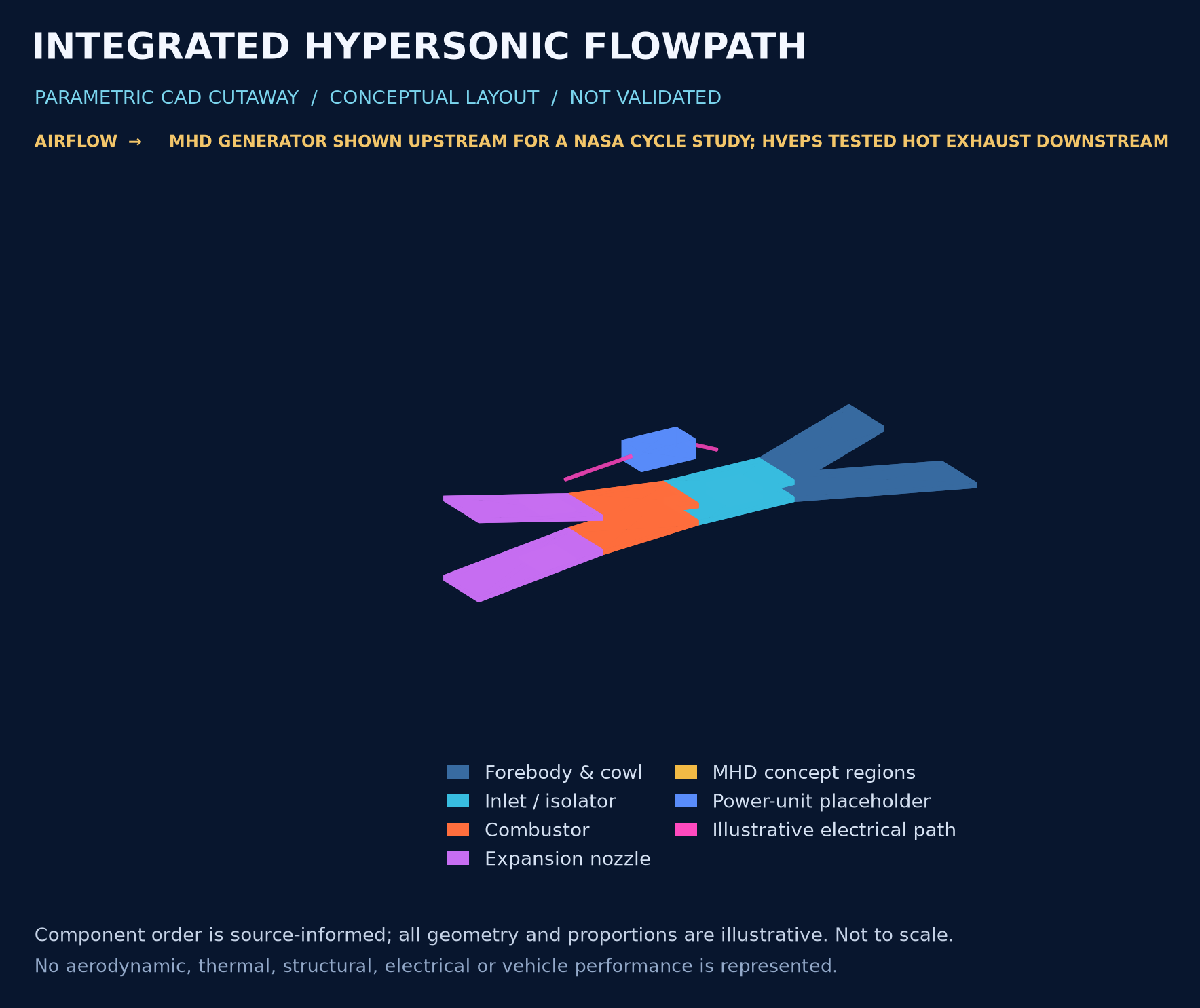
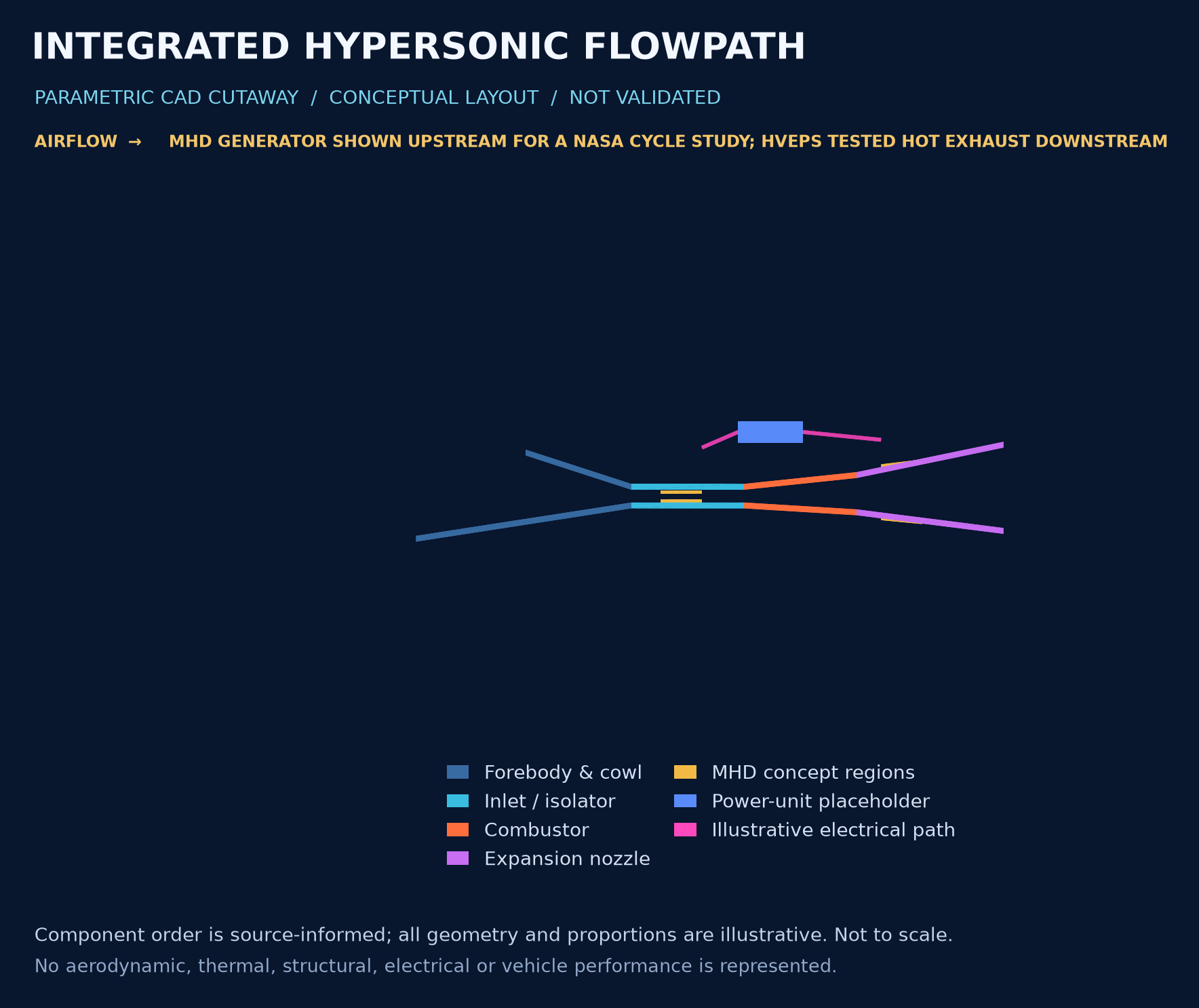
What a five-year-old can see: air comes in from the left, passes through several differently shaped spaces, mixes with fuel in the middle, then leaves at the right. The yellow pieces mark places where a research idea would try to take energy from the gas and add some electrical energy back later.
This is an editable parametric CAD teaching model, not a validated engine or aircraft. The component order is informed by published scramjet and MHD-cycle descriptions; every shape and proportion in this model is illustrative. CAD exchange units are used for compatibility and must not be read as a proposed vehicle scale. Magnetic-field hardware, plasma and seeded working gas are intentionally omitted. The model calculates no airflow, combustion, plasma conductivity, heat transfer, material stress, thrust, net power or flight performance.
Do not confuse two arrangements: the gold generator markers here are placed upstream of combustion to echo the simplified cycle analyzed in the 2000 NASA study. The HVEPS ground experiment used a generator downstream of the combustor to take energy from hot exhaust. These are different system layouts and evidence. HVEPS reported a component test; it did not demonstrate this complete inlet-to-generator-to-accelerator cycle in flight. NASA's modeled cycle study · General Atomics' account of the HVEPS test · Air Force account of the HVEPS test.
For the integrated scramjet arrangement, see NASA's X-43A research overview.
Files from this model: editable STEP solid assembly · STL viewing mesh · parametric CAD source · component list
The CAD does not show a gas-recirculation loop. Electrical extraction and later re-input are separate processes, and any net benefit depends on losses and integration that this geometry does not model.
At hypersonic speed, the aircraft and engine cannot be treated as unrelated shapes. The forebody helps prepare incoming air; the underside accommodates the engine, and aft surfaces participate in expansion. This motivates an integrated layout. The drawing is not a mathematically derived waverider and has no demonstrated optimum. NASA's integrated X-43A research.
A scramjet uses atmospheric oxygen and retains supersonic flow in its combustion region. It has no rotating compressor-and-turbine core like a conventional turbojet. The airflow, fuel mixing, combustion and nozzle must work together. This is one candidate architecture, not a claim that every hypersonic mission requires it. NASA's X-43A research.
Heating affects the nose, leading edges, structure and engine. The design must balance aerodynamic shape with heat load and material response; an infinitely sharp edge is not a practical thermal solution. The highlighted panels locate a design concern, not a calculated temperature map. NASA's materials and structures review.
The potential civilian benefit is faster long-distance travel or high-speed atmospheric research. Practical usefulness still depends on range, payload, total energy use, noise, sonic boom, heating, reliability and cost. A short experimental flight is not proof of an economical transport service.
FLIGHT EVIDENCE / TEST THE HEAT MODEL
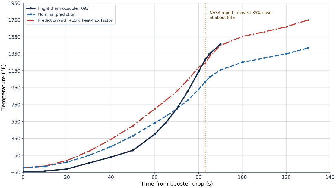
Simple version: Engineers predicted how hot different parts would get. On one forward part of the X-43A's vertical tail, a sensor became hotter than the extra heating allowed for in the design case. The cause was not solved. That is why flight sensors and careful follow-up matter.
During the X-43A's 27 March 2004 Mach-7 research flight, thermocouple T093 measured a thin-skin area near the front of the vertical tail. NASA's report says temperatures at T093 and a second sensor, T094, rose above the prediction that included a +35% heat-flux factor at about 83 seconds after booster drop. The paper describes this as an anomaly in an otherwise generally conservative set of predictions, not evidence that every hypersonic heat model fails.
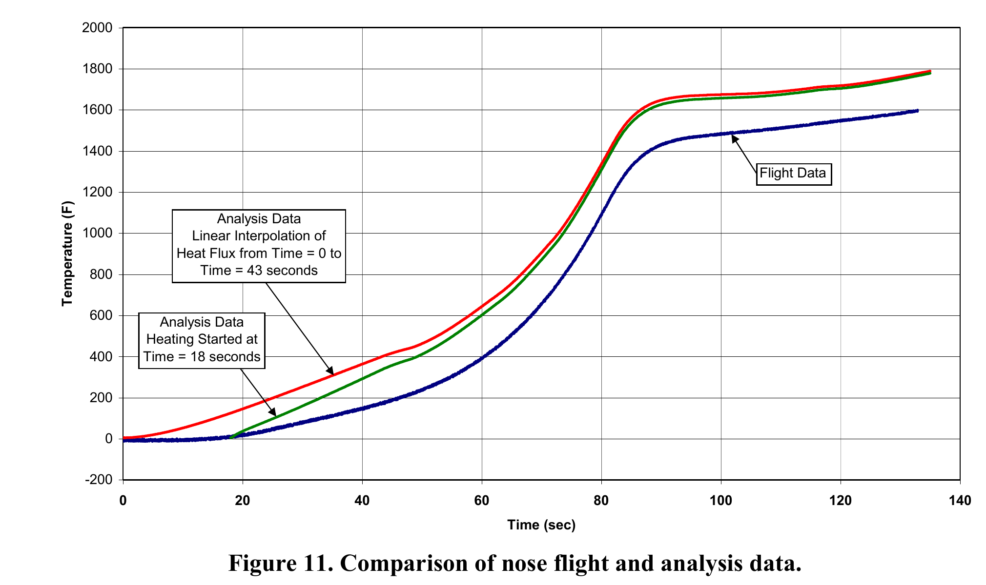
Simple version: A temperature sensor near the nose stayed almost level for the first 18 seconds. The first computer model began adding heat from the moment the booster dropped, so it predicted a warmer nose early on. NASA reran the model with no heating during those first 18 seconds. That changed the early part of the curve, but the two model curves were nearly together by about 70 seconds.
| Evidence | Reported result | Limit |
|---|---|---|
| Flight sensor | One nose thermocouple showed virtually no temperature increase during the first 18 seconds. | It sat on a butt line 0.50 in off the centerline and 0.50 in aft of the leading edge; it did not measure the leading-edge tip. |
| Original analysis | Heat flux was linearly interpolated from booster drop at 0 s to the first aerothermal heating data near 43 s. | This implied some early heating at transonic and low-supersonic speeds; the authors called it conservative. |
| Postflight rerun | The rerun assumed no heating during the first 18 s, then used the same later aerothermal data points. | The changed assumption improved the early comparison; NASA says the curves were virtually the same by about 70 s and that final/max temperature was relatively insensitive to the early heating for these thin parts. |
| Interpretation | This is a useful check of the initial-heating assumption against a nose temperature trace. | NASA says no additional effort had been made to correlate the nose flight data with the analysis at the time of publication. No thermocouples were installed in the carbon-carbon leading edge. It does not validate every nose or leading-edge temperature prediction. |
Read this beside the T093 vertical-tail case above: one example shows a forecast crossing at a local sensor; the other shows how changing an early heat-flux assumption shifts a separate nose trace. They concern different sensors and model questions. Temperature is what these thermocouples measured; it is not a direct heat-flux measurement. NASA’s instrumentation limitation, PDF p. 15.
The NASA authors proposed that a local flow pattern and shock interaction might be adding heat that the engineering model did not capture. They tried artificial increases to the shock angle and heating augmentation, but these did not reproduce the flight response. The paper leaves the cause unresolved and identifies more rigorous flow analysis as future work. This is a useful research result: a specific measurement showed where the model needed further investigation. It is not proof of one confirmed cause.
A different NASA study addressed materials for the X-43A Mach-10 flight. Before that flight, analysis predicted that the nose tip might approach 4,000 °F. Researchers tested 13 material systems in an arc-jet facility under a simulated 130-second heating environment, then selected carbon-carbon leading edges for the flight hardware. The report says seven of eleven parts received the full SiC/HfC three-layer coating; the four chine parts received only the first two layers. NASA reports that the leading edges performed as expected on that single short research flight. The paper does not publish a complete numerical result for every candidate material, so it cannot support an honest chart ranking all 13. The predicted 4,000 °F, Mach-7 T093 flight sensor and Mach-10 ground material tests are different evidence. A 2004 follow-up arc-jet test then found unexpected erosion on both short-span carbon-carbon models. The study changed the leading-edge nose radius from 0.030 to 0.050 inch for the flight design; it explicitly says the erosion mechanism was not proven. The 5.89-inch test span fit the facility limit, but the authors say it could not reproduce the full-scale buckling and shear stresses. The Mach-10 flight was a single short research flight, not a reusable-aircraft qualification. NASA Mach-10 leading-edge study record · NASA study PDF.
Why people should care: comparing models with flight sensors helps engineers find local heating that a broad safety margin may miss. Arc-jet tests can help select materials before flight. Neither result by itself qualifies a reusable passenger aircraft or proves the proposed MHD energy-recovery system.
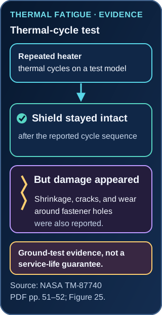
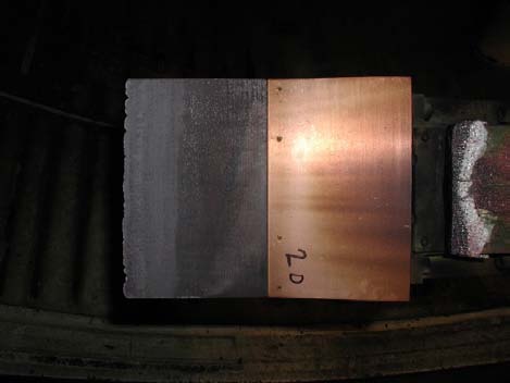
The simple version: imagine warming and cooling a metal lid again and again. It may stay in one piece but develop small cracks near the holes that hold it down. Engineers check for damage as well as whether a heat shield stays together.

What was observed: a historical ground experiment repeatedly heated and cooled a heat-shield test model. The review reports 20,040 thermal cycles; the original report abstract rounds this to about 20,000. The shield stayed intact, but shrinkage, cracks, wear around fastener holes and reduced ductility were also reported. These cycles were not flights or a demonstrated service life.
NASA TM-87740 distinguishes several kinds of evidence. Figure 23 compares a shielded panel's ground-test temperature response with a calculated unshielded response. Figure 24 compares measured average temperatures with one-dimensional transient predictions during a simulated loss-of-cooling heating sequence; its unprotected-panel comparison is also calculated. Figure 25 summarizes thermal cycling and damage. None is a flight demonstration of a complete propulsion system.
This page summarizes the review and the original fatigue report's abstract. It also provides a separate approximate graph-reading redraw and downloadable readings. Those extracted values are not raw test data, and the source does not establish a measurement uncertainty budget. The original curves and apparatus details remain available in the source report.
Shore (1986), NASA TM-87740 · Review PDF: Figures 23–25 on physical pages 48, 50 and 52 · Webb, Clark and Sharpe (1985), original fatigue-test report and abstract.
GROUND TEST / SIMULATED LOSS OF COOLING
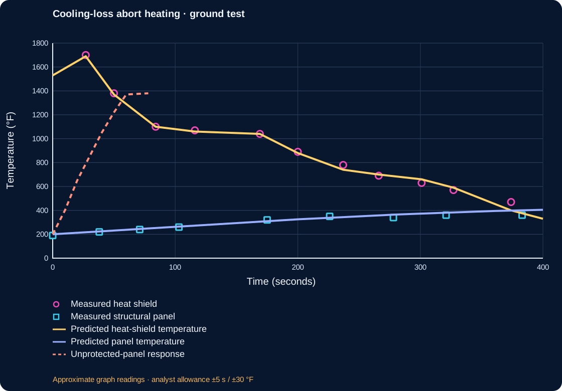
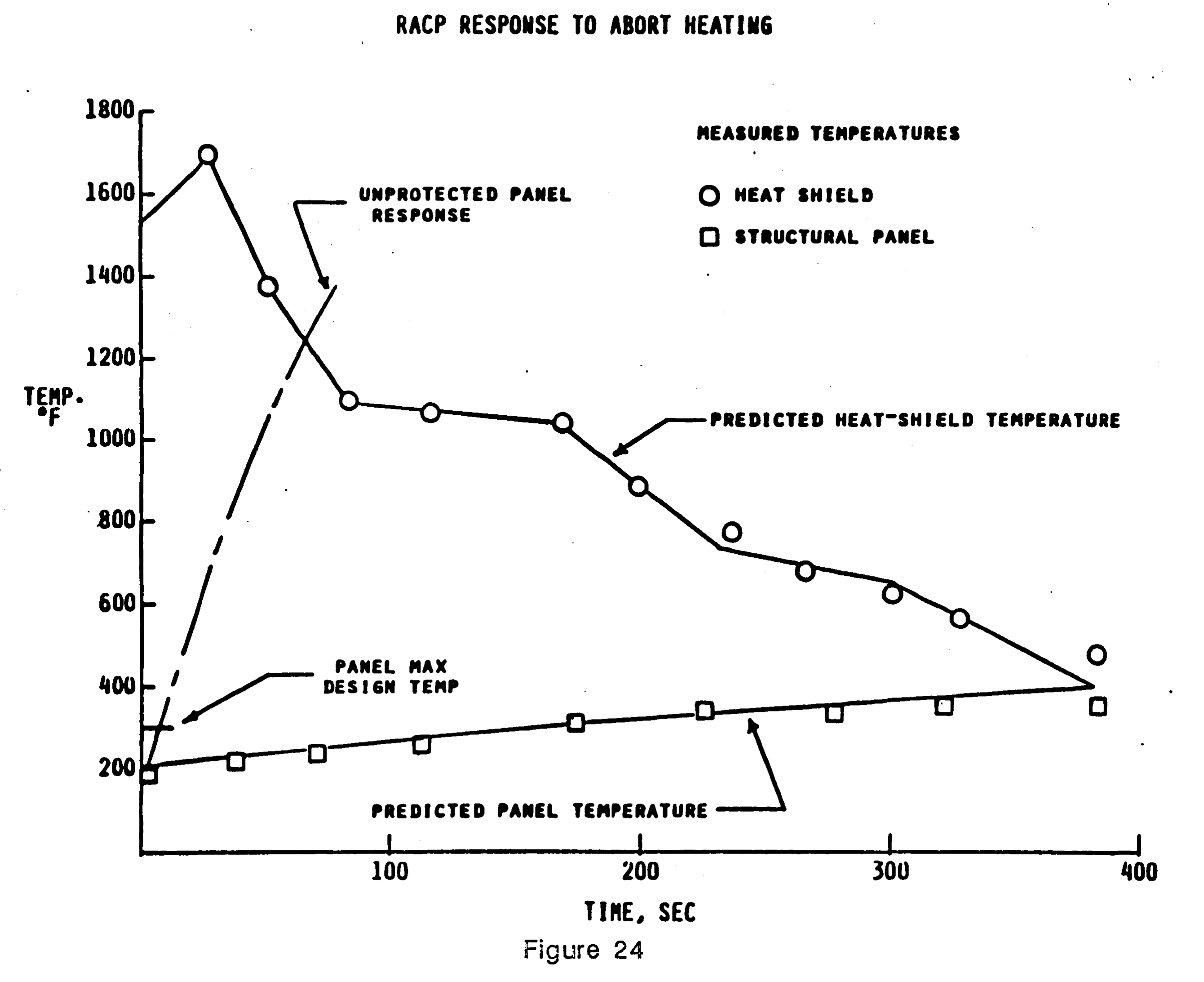
Simple version: imagine a hot shield protecting a cooler panel. After a simulated loss of coolant, engineers tested a reduced-heating abort path intended to let the aircraft slow down. The shield became very hot, while the panel warmed more slowly. Engineers measured both parts, then compared those measurements with a computer calculation.
The source plot uses circles for measured heat-shield temperatures and squares for measured structural-panel temperatures. The labeled predicted shield and panel temperatures are calculated curves. The dashed line is a calculated unprotected-panel response, not another sensor measurement. The experiment is a ground test with a simulated abort heating sequence; it is not X-43A flight data and does not test an MHD generator.
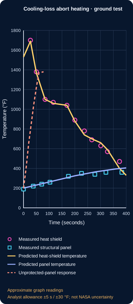
| Trace | Time (s) | Temperature (°F) | Trace class |
|---|---|---|---|
| Measured heat shield | 27 | 1700 | measured_marker |
| Measured heat shield | 50 | 1380 | measured_marker |
| Measured heat shield | 84 | 1100 | measured_marker |
| Measured heat shield | 116 | 1070 | measured_marker |
| Measured heat shield | 169 | 1040 | measured_marker |
| Measured heat shield | 200 | 890 | measured_marker |
| Measured heat shield | 237 | 780 | measured_marker |
| Measured heat shield | 266 | 690 | measured_marker |
| Measured heat shield | 301 | 630 | measured_marker |
| Measured heat shield | 327 | 570 | measured_marker |
| Measured heat shield | 374 | 470 | measured_marker |
| Measured structural panel | 0 | 190 | measured_marker |
| Measured structural panel | 38 | 220 | measured_marker |
| Measured structural panel | 71 | 240 | measured_marker |
| Measured structural panel | 103 | 260 | measured_marker |
| Measured structural panel | 175 | 320 | measured_marker |
| Measured structural panel | 226 | 350 | measured_marker |
| Measured structural panel | 278 | 340 | measured_marker |
| Measured structural panel | 321 | 360 | measured_marker |
| Measured structural panel | 383 | 360 | measured_marker |
| Predicted heat-shield temperature | 0 | 1530 | calculated_curve |
| Predicted heat-shield temperature | 27 | 1690 | calculated_curve |
| Predicted heat-shield temperature | 50 | 1370 | calculated_curve |
| Predicted heat-shield temperature | 84 | 1100 | calculated_curve |
| Predicted heat-shield temperature | 116 | 1060 | calculated_curve |
| Predicted heat-shield temperature | 169 | 1040 | calculated_curve |
| Predicted heat-shield temperature | 200 | 880 | calculated_curve |
| Predicted heat-shield temperature | 237 | 740 | calculated_curve |
| Predicted heat-shield temperature | 266 | 700 | calculated_curve |
| Predicted heat-shield temperature | 301 | 660 | calculated_curve |
| Predicted heat-shield temperature | 327 | 590 | calculated_curve |
| Predicted heat-shield temperature | 374 | 400 | calculated_curve |
| Predicted heat-shield temperature | 400 | 330 | calculated_curve |
| Predicted panel temperature | 0 | 200 | calculated_curve |
| Predicted panel temperature | 40 | 225 | calculated_curve |
| Predicted panel temperature | 80 | 250 | calculated_curve |
| Predicted panel temperature | 120 | 275 | calculated_curve |
| Predicted panel temperature | 160 | 300 | calculated_curve |
| Predicted panel temperature | 200 | 325 | calculated_curve |
| Predicted panel temperature | 240 | 345 | calculated_curve |
| Predicted panel temperature | 280 | 365 | calculated_curve |
| Predicted panel temperature | 320 | 380 | calculated_curve |
| Predicted panel temperature | 360 | 395 | calculated_curve |
| Predicted panel temperature | 400 | 405 | calculated_curve |
| Unprotected-panel response | 0 | 200 | calculated_curve |
| Unprotected-panel response | 10 | 400 | calculated_curve |
| Unprotected-panel response | 20 | 650 | calculated_curve |
| Unprotected-panel response | 30 | 850 | calculated_curve |
| Unprotected-panel response | 40 | 1050 | calculated_curve |
| Unprotected-panel response | 50 | 1220 | calculated_curve |
| Unprotected-panel response | 60 | 1370 | calculated_curve |
| Unprotected-panel response | 78 | 1380 | calculated_curve |
The figure's x-axis is time in seconds and the y-axis is temperature in degrees Fahrenheit. It shows average component temperatures under the reported ground-test sequence. Its labeled one-dimensional transient calculations are not instrument readings. The plot does not provide raw time-series data, error bars, or a measured uncertainty budget. The accompanying dataset consists of approximate graph readings with a stated project allowance for pixel/axis reading; that allowance is not experimental uncertainty. It cannot establish full-vehicle thermal safety, flight performance, reusable service life, or propulsion-system energy recovery.
How this could help people: repeated-use testing helps reveal damage that a single successful heating test can miss. That evidence can inform inspection and durability research for reusable thermal protection. It does not certify this concept for carrying passengers.
Simple version: Engineers compared what the aircraft did in flight with what their computer models and wind-tunnel tests predicted. The pictures show where the curves look similar or different. They do not give enough readable numbers to measure every difference from the image.
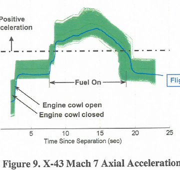
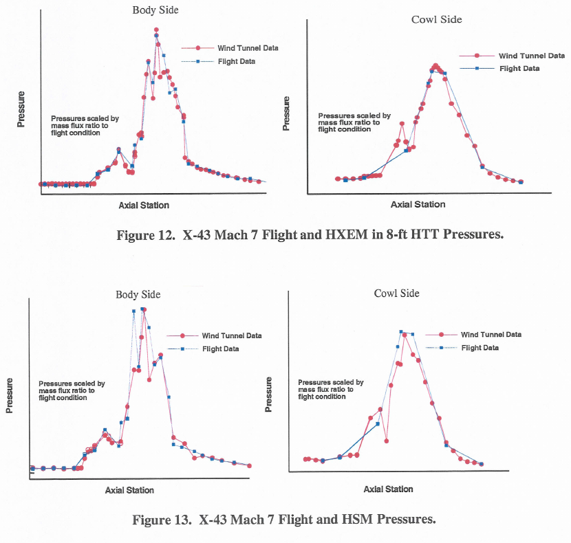
The X-43A flight, preflight calculation and ground-facility traces are different kinds of evidence. The NASA paper plots them together for comparison, but several axes have no readable numerical graduations. The faithful figures below preserve the source plots without tracing them into invented data. In Figure 9, the green Monte Carlo band shows model runs; it is not the flight sensor's uncertainty. Put simply, engineers run the model many times with slightly different assumed inputs. The spread helps them see how sensitive the prediction is to those assumptions; it is not a measured range around the flight data.


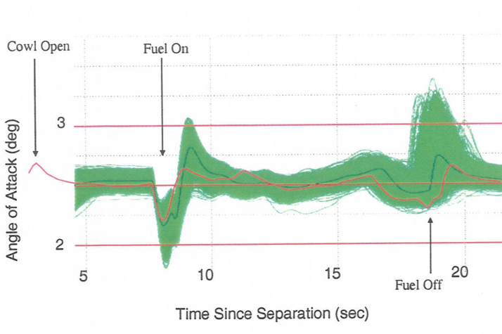
Simple idea: This graph compares the aircraft's nose angle with the flight team's computer predictions as the engine changed state.
Scientific reading: NASA's text says the target angle was 2.5 degrees during the cowl-open portion. The red line is the flight trace, the thin green line is the nominal preflight path and the green band contains Monte Carlo model runs. That band describes model variation, not sensor uncertainty. We retain the published graph and do not digitize curve values.
Source: Ferlemann et al., Figure 8, NASA NTRS 20050215122 (public use permitted). NASA PDF, p. 5.
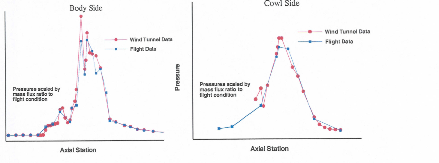
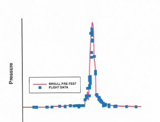
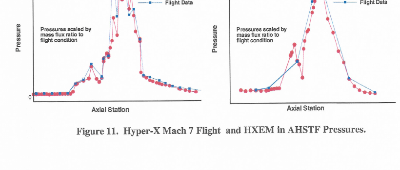
Simple idea: Many small sensors measure how air presses on different parts inside the engine. Engineers compare those flight readings with a wind-tunnel test.
Scientific reading: Body-side and cowl-side traces are shown separately. HXFE pressures are scaled by mass-flux ratio to flight conditions. Neither vertical axis has usable numeric graduations, so the plot supports a comparison of shapes, not absolute pressure or a calculated error.
Source: Ferlemann et al., Figure 14, NASA NTRS 20050215122 (public use permitted). NASA PDF, p. 8.
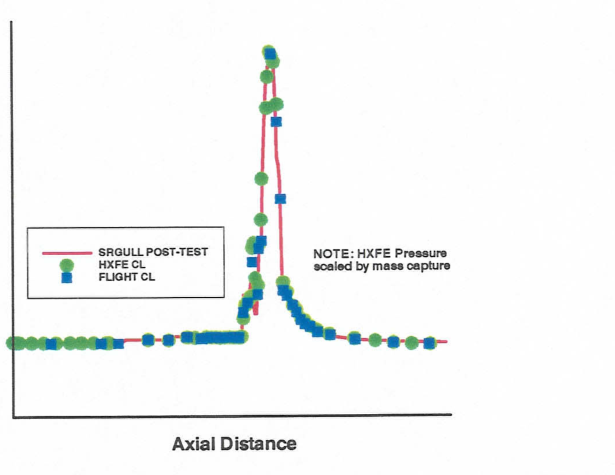
Simple idea: After the flight, engineers changed parts of their computer model to better match what the sensors and flight analysis showed.
Scientific reading: NASA reports using the best-estimated trajectory and three-dimensional CFD updates to mass capture and momentum. They varied combustion efficiency to match isolator/combustor pressures and flight-estimated thrust. HXFE ground-test pressure was scaled by mass capture. This is a post-test fit, not a blind prediction or an independent measurement of thrust from this graph. Its axes are not numerically graduated.
Source: Ferlemann et al., Figure 15, NASA NTRS 20050215122 (public use permitted). NASA PDF, p. 8.
What this can and cannot show: these published comparisons help explain how flight evidence, wind-tunnel tests and predictions are checked against one another. They do not test an MHD generator, a closed energy-recovery loop, or a passenger aircraft. Source: S. M. Ferlemann, C. R. McClinton, K. E. Rock & R. T. Voland, “Hyper-X Mach 7 Scramjet Design, Ground Test and Flight Results,” AIAA 2005-3351, Figures 8–15. NASA NTRS record and use/rights metadata · NASA report PDF.
HOW THE EVIDENCE BUILDS / DIFFERENT TESTS ANSWER DIFFERENT QUESTIONS
Simple version: Scientists test an engine piece in a wind tunnel, carry another engine to fast speed on a rocket, and later fly a small uncrewed research aircraft. They also heat materials in a separate test facility. Each test gives a clue; they are not all tests of one complete machine.
These studies form a useful learning path, not a matched campaign: they used different hardware, facilities, speeds, and measurements. Follow each result only as far as its test allows.
The forebody and inlet guide incoming air toward the engine. The Site's CAD is a teaching geometry, not a validated flow solution or optimum. It explains what designers must coordinate; it does not predict what the aircraft would do.
A NASA Mach-6 tunnel study measured a separate inlet at four angles of attack. Its report gives about 78% total-pressure recovery and 99% adiabatic kinetic-energy efficiency for that test article. These are two different measures from a component test; they do not validate this CAD, another engine, or a complete flight vehicle. NASA TN D-7998 record · Figure 12(c), PDF p. 58.
The 1998 CIAM experiment carried an axisymmetric dual-mode engine under a rocket booster over roughly Mach 3.5–6.4. At the highest-Mach point, combustion turned much of the combustor flow subsonic; the report discusses inlet changes and a control-sensor problem. The engine was carried to the condition, not a self-accelerating scramjet aircraft. CIAM/NASA flight and ground-test study · NASA primary record · Conclusion and evidence limit, PDF p. 8.
The Mach-7 X-43A flight tested an airframe-integrated scramjet over a brief research flight. NASA emphasizes how predicted propulsion behavior compared with flight, wind-tunnel, and computational methods. The source is an AIAA conference preprint in NASA's record, not a demonstration of routine transport or the proposed MHD system. View the Mach-7 source figures · NASA NTRS record · Figs. 8–9, PDF p. 5.
During the Mach-7 flight, thermocouples T093 and T094 on the vertical tail exceeded the prediction that already included a 35% heat-flux factor, at about 83 seconds. Those are measured temperatures, not direct heat-flux readings; the cause remained unresolved. This tests a thermal prediction at particular instrumented locations, not every part of a vehicle. The approximately 83-second T093 event occurred before X-43A separated from its Pegasus booster at about 95 seconds after drop; the plotted trace ends near 90 seconds. It therefore records local heating during booster ascent, before the later cowl-open and fuel-on events in the engine-flight timeline, and does not measure powered scramjet heating. Read the sensor/model comparison · NASA thermal-analysis report · NASA engine-flight timeline (cowl-open and fuel-on relative to separation) · Download local source copy (scanned PDF) · T093/T094 discussion, PDF p. 20 · Figure 19, PDF p. 21.
Separate arc-jet campaigns screened 13 material systems. A 2004 follow-up found erosion on two small-span test articles; the team changed the nose-tip radius and leading-edge design. The facility's span limit could not reproduce full flight-span stresses. NASA reports that the selected leading edges performed as expected on one short Mach-10 research flight, not that they were qualified for reuse. This is a different vehicle and heat-test campaign from the Mach-7 thermocouples. NASA Mach-10 materials paper and rights record · Span limit, unproven erosion cause and redesign, PDF p. 6 (printed p. 7).
What the whole chain does not prove: it does not combine these components into one validated hypersonic aircraft, establish commercial usefulness, or test MHD energy generation and reinjection. Those require their own matched measurements, complete force/energy balances, and independent validation.
Define the intended flight regime, payload, range and operating duration. Then assess the coupled airflow, combustion, heating, structure and control, including the acceleration system. Wind-tunnel, propulsion and material tests would be required to validate predictions. No maximum speed, endurance, thermal margin or optimal geometry is claimed here.
ENERGY RECOVERY / WHAT CAN COME BACK?
A useful starting question is: can energy in hot, fast gas be put back to work? The answer depends on which energy is collected, where it goes and what it costs to collect it. Heat transferred through a wall, compression of incoming air and power extracted from an outgoing jet are different processes.
A concrete starting point is regenerative cooling. Incoming fuel flows through passages beside hot engine walls, absorbs some heat and then enters the combustor. The fuel helps cool the structure and carries that heat back into the engine's energy flow. NASA has studied both direct fuel cooling and separate coolant loops that transfer heat to fuel. NASA · Convectively cooled hypersonic structures.


A conventional gas-turbine engine already uses a turbine to extract work and drive its compressor. A scramjet normally has no such rotating core in its main supersonic flow. A separate cooling circuit is a different design question. NASA · Gas-turbine cycle.
A coolant can circulate internally, but the air-breathing engine still exchanges momentum with the surrounding air. Gas circulating entirely inside an otherwise isolated aircraft cannot, by itself, produce sustained net thrust. Burned exhaust also does not become fresh fuel merely by cooling or slowing it.
HYPERSONIC INLET / FOLLOW THE ENERGY
An inlet can slow captured air, raising its static temperature; compression can also raise its static pressure. In an ideal adiabatic inlet with no shaft work, it does not create energy: the flow's kinetic energy becomes static enthalpy while total enthalpy stays constant. Real shocks, friction and mixing lower total pressure, which reduces the flow quality available downstream. A pressure rise is not electricity, and the pressure-recovery percentage below is an assumption, not energy recovered.
Supersonic outlet state (scramjet-style combustor condition)
The stream loses kinetic energy as its static enthalpy rises by the same amount.
At an assumed 1 kg/s through-flow, the stream momentum-flux change is −401.0 N. This is not vehicle thrust: inlet-wall and pressure forces, captured or spilled mass, and matched downstream conditions are not modeled.
Model: ht = cpT + V²/2 = constant; Tt = T + V²/(2cp). Static outlet pressure follows from the selected outlet Mach number and assumed total-pressure recovery.
Assumptions: one-dimensional steady flow; ideal air with γ = 1.4 and cp ≈ 1005 J kg⁻¹ K⁻¹; freestream static state fixed at 220 K and 4.0 kPa as an illustrative high-altitude-like reference, not a specified trajectory; no wall heating or shaft work in this model. Real hypersonic gas can have temperature-dependent properties and chemical effects, and real inlets add shock, viscous, mixing and geometry constraints.
Combustor condition: below Mach 1 is a subsonic (ramjet-style) state; above Mach 1 is a supersonic (scramjet-style) state. Real dual-mode engines do not switch at one universal slider value: inlet state, heat addition, geometry and thermal choking all matter. See NASA's dual-mode analysis.
Pressure recovery is a separate track. The slider independently assumes how much freestream total pressure remains after the inlet; the model does not predict it from geometry. One NASA analysis reported about 70% for particular Mach 4–5 inlet configurations, which is a case result, not a universal value. NASA's inlet study.
Important boundary: the calculated outlet pressure is a thermodynamic state from the chosen Mach number and assumed pressure recovery. This model has no inlet area, captured-air mass flow or continuity equation, so it does not describe a matched operating point and cannot predict power or thrust.
For a young reader: Engineers put a model air inlet in a very fast wind tunnel and tilted it a little. They measured the pressure and temperature in several places. At these test settings, about four-fifths of a particular pressure measure remained through the narrow throat, averaged over its area. That measure is not a percentage of the air's energy. The study separately reported 99% adiabatic kinetic-energy efficiency. Those are different results with different meanings: neither says that 78% or 99% of the air's energy became electricity.

The report describes a fixed-geometry swept external-internal compression inlet tested at Mach 6, test-section Reynolds number 1.55 × 10⁷ per metre, stagnation pressure 20 atmospheres, stagnation temperature 500 K, and angles of attack −5°, 0°, 3°, and 5°. Pitot- and static-pressure surveys were made in the throat, alongside wall pressure and surface-temperature measurements. Boundary-layer bleed was used on the centerbody and cowl. The report calls ηD,max = 0.91 its most realistic limiting-recovery setting for the data reduction; this setting is not the measured average. Figure 12(c) shows the arithmetic average of recovery over the throat area, not the separate mass-weighted recovery quantity discussed elsewhere. Surface temperatures were measured, but this graph does not plot heat flux or a coolant-energy balance. It is a ground test of one inlet component, not a flight test or whole propulsion system. Full methods and boundaries.
Each result answers a different question, under a different boundary. Adding their numbers together would mix an ideal calculation, separate experiments and an illustrative ledger.
| Evidence or calculation | What it tells us | What it does not provide |
|---|---|---|
| Ideal inlet, Mach 5 to Mach 2 | About 515.7 kJ/kg of flow kinetic energy becomes static enthalpy in the stated perfect-gas model. | Captured mass flow, inlet area, electrical output or an actual engine operating point. |
| NASA Mach 6 inlet wind-tunnel test | One tested inlet's approximate throat pressure recovery and separately reported adiabatic kinetic-energy efficiency. | An MHD generator, electrical bus, accelerator, nozzle force or vehicle drag. |
| HVEPS MHD generator ground test | Electrical generation from a hot ground-test exhaust stream; published summaries describe different output details. | A matched inlet measurement, generator-to-accelerator loop, full engine power balance or flight thrust gain. |
| NASA Ames MHD-accelerator channel tests | Two laboratory runs reported approximately 27% and 38% increases in cross-section-averaged flow velocity. A later numerical paper predicted about 26% for Run 15 and 30–31% for Run 16. | An electrical generator, recovered-energy loop, vehicle net thrust, or flight benefit. The channel accelerator used applied electrical and magnetic fields under brief hot-flow conditions. |
| NASA MHD-bypass cycle analysis | A simplified thermodynamic model couples a generator and accelerator, including selected aerodynamic losses and process efficiencies. | A built or flown integrated engine; its authors report that non-isentropic MHD losses hamper overall performance. |
| Illustrative post-combustor thrust ledger | A momentum-only sensitivity for its declared fixed-flow assumptions. | Changing mass flow, measured nozzle pressure thrust, geometry, coupled inlet losses or a validated complete cycle. |
The child-simple version: A magnet can help hot, electrically conducting gas make electricity. But the magnet, cooling equipment, wires and support frame all add weight. A 2026 paper estimates several possible arrangements on paper. It is a design study, not a tested aircraft engine.
The paper compares rare-earth permanent magnets and two high-temperature-superconductor arrangements. Its channel-power estimate uses Pd = σv2B2/4, then assumes a 1000 m/s flow, 10 S/m conductivity, and estimates for structures, cooling, electrodes and seeding. The resulting kilowatts and kW/kg are model-based design estimates, not measured net aircraft-bus power.
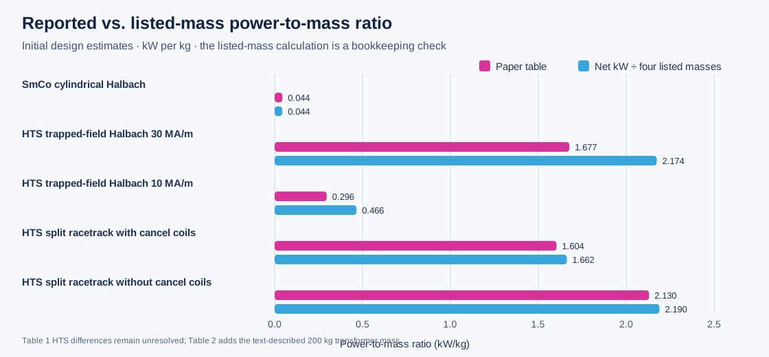
One unit label needs care: the paper's Table 1–2 heading says volumetric power density in W/m³, but its listed values (2, 82, 103…) match megawatts per cubic metre when calculated from the paper's own equation and inputs. For example, σ = 10 S/m, v = 1000 m/s and B = 5.71 T give about 81.5 MW/m³, consistent with the table's rounded 82. This appears to be a table-unit-label mismatch; we retain and explain it rather than silently changing the source.
| Proposed magnet arrangement | Paper's power estimate (kW) | Paper's kW/kg | Sum of four printed mass columns (kg) | Power ÷ printed mass sum (kW/kg) | Audit note |
|---|---|---|---|---|---|
| SmCo cylindrical Halbach | 207 | 0.044 | 4,733.8 | 0.0437 | Matches after rounding. |
| HTS trapped-field Halbach, 30 MA/m | 7,336 | 1.677 | 3,374.4 | 2.174 | Reported ratio implies about 1,000 kg additional denominator mass; not located in Table 1's stated assumptions. |
| HTS trapped-field Halbach, 10 MA/m | 812 | 0.296 | 1,743.5 | 0.466 | Also implies about 1,000 kg additional denominator mass; unresolved. |
| HTS split-racetrack, cancel coils | 9,243 | 1.604 | 5,561.1 | 1.662 | Adding the separately described 200 kg transformer pack gives about 1.604. |
| HTS split-racetrack, no cancel coils | 15,590 | 2.130 | 7,119.9 | 2.190 | Adding the separately described 200 kg transformer pack gives about 2.131. |
The authors estimate 300 kg of common support for cylindrical Halbach arrays; superconducting trapped-field cases also assume a 200 kg cryostat and 24 coolers totalling 74.4 kg. Electrodes, leads and power conditioning are scaled at 0.25 kg/kW. The RF interface is estimated at 60 kW and 200 kg; chemical seeding is assigned 150 kg. The paper says RF heating is expected to improve extraction, but the tables do not show a reconstructable electrical debit for its 60 kW draw. So the label “Net Power Est” cannot be independently interpreted as a closed vehicle-bus balance from the published table alone.
The paper also says its current stainless-steel support design is unlikely to survive full magnet excitation. The authors defer electrode optimisation and MHD flow simulation until the magnet structure is revised. These are valuable early design-space calculations, while the hardware, structural mass, power accounting and integrated flow/force balance remain open. Paper DOI · Author-uploaded full text.
Download graph · SVG · Download transcribed values and checks · CSV · Reproduce the figure · Python
Simple version: One report described a test that was still being built. A later paper reported a short ground test. Another paper compared computer calculations with selected test measurements. Those percentages answer different questions, so they do not make one continuous performance curve.

The separate NASA TM-2001-210922, “Facility and Conductivity Measurements,” is cited in the 2004 paper, but I did not find a distinct public NTRS record or download under its exact number during this bounded search. The 2001 four-page NASA preprint linked above is a separate document and must not be presented as that TM. None of these sources reports an integrated generator-to-accelerator hypersonic vehicle balance or net thrust.
These studies are different kinds of evidence. A measured component output, a modeled cycle, and a facility design prediction answer different questions. This matrix records each study’s boundary, available inputs, and uncertainty status; it does not rank their performance or combine unlike quantities.
| Case and evidence type | Boundary and reported result | Inputs and uncertainty available | What it supports—and what it cannot establish |
|---|---|---|---|
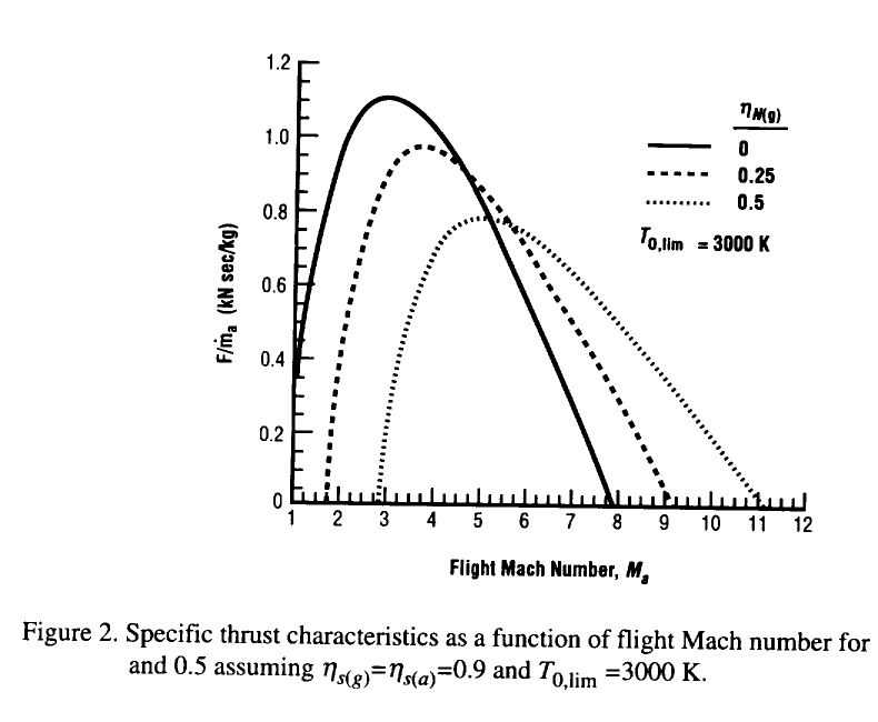
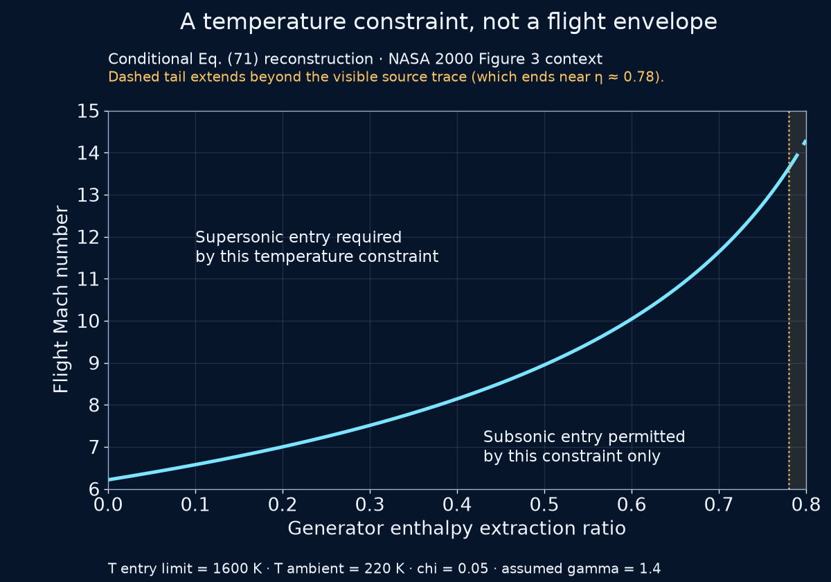
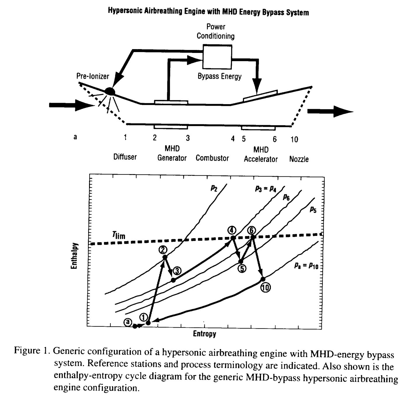
| NASA 2000 cycle model Analytical cycle | Simplified inlet → generator → combustor → accelerator/nozzle; output depends on chosen efficiencies and extraction/addition assumptions. | Report equations and figures are public; no pointwise source table, code or statistical uncertainty package was exposed in the inspected record. The earlier discrepancy claim was withdrawn because curve identity was not established; the approximate figure readings do not establish a mismatch with NASA numerical results. | Supports a bounded equation-based reconstruction. Does not validate hardware or yield a matched whole-vehicle comparison. |
| NASA 2001 ionizer case Analytical model | One modeled case compares 827 MW ionizer demand with 151 MW gross generator output, assuming a 100%-efficient ionizer. | Table 1 is transcribed from the retained, checksummed report PDF; no measurement or full-system uncertainty budget. | Supports the case-specific ~5.48 ratio. Does not prove universal failure, measured performance or net aircraft thrust. |
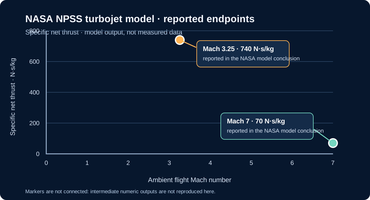
| Benyo 2010 NASA/TM—2010-216734 Preliminary 1-D turbojet-cycle analysis; AIAA-2010-0232 | Predicts up to 420 N·s/kg specific thrust for selected Mach-2.0–3.5 cases at 1–5 T and models a possible operating range to Mach 7. | The NASA report calls its findings preliminary and identifies simplifications: point-to-point 1-D analysis, bypass-energy accounting only, fixed areas, and no iterative matching of higher-Mach conditions. It is not an engine test. | Early calculated feasibility result, not demonstrated performance. Distinct from the later June 2010 AIAA-2010-4301 flow-matching conference paper and the 2011 final NPSS report. NASA/TM PDF, abstract and limits at printed pp. 1–2 · Local primary PDF. |
| Benyo 2011 final NPSS report Coupled turbojet-cycle simulation | Pre-ionizer, MHD generator, turbojet, second pre-ionizer and accelerator. Across Mach 3.25–7, selected cases report 45–90 MW extraction and positive specific net thrust of 740 to 70 N·s/kg. | Model assumes 90% generator isentropic efficiency, 2.5 T and prescribed 2–5.5 S/m conductivity; pointwise NPSS deck and statistical uncertainty are not provided. The distinct June 2010 AIAA-2010-4301 flow-matching paper uses a 10 m generator and reports 1 mho/m for its pre-ionizer case (not a measured generator conductivity); its outputs are not mixed here (conference paper PDF). | Demonstrates that one modeled turbojet cycle predicts positive thrust under its assumptions. Does not establish scramjet performance, tested hardware, magnetic-system mass/cooling/drag or vehicle-level benefit. Final report PDF. |
| Schneider 2011 annular Hall-MHD cycle Preliminary 1-D axisymmetric simulation | At Mach 7 / 30 km, the iterated cycle calculates 185 N·s/kg specific thrust; its generator extraction is 1.6 MJ/kg and, after ionizer allocation, about 1.4 MJ/kg is passed to the accelerator. | The generator case uses 3 m, 5 T / 5 S/m; the accelerator case uses 3 m, 5 T / 1 S/m. Calculated efficiencies are 84% and 81%. Required ionization is estimated 2–3 orders above the cited discharge estimate. | Model only. The report calls for higher-dimensional calculations and generator/accelerator experiments; it does not demonstrate a viable integrated system. NASA report PDF. |
| Riggins 2004 Modeled cycle; abstract-level here | Thermally balanced MHD-bypass versus conventional scramjet simulations, Mach 8–12.2. | Abstract-level result in this audit; full numerical data and uncertainty details were not inspected or reproduced. | Supports reporting a configuration-specific modeled penalty. No exact reproduction or universal conclusion. |
| Kaminaga 2005 Quasi-1D model | Models generator braking alongside combustion pressure, wall friction and accelerator work; Figure 12 reports normalized net-thrust trends. | Full article graph available; project readings are approximate, with image-reading tolerance only. Source pointwise data and a complete model-uncertainty budget were not found. | Supports a source-attributed example of competing calculated force contributions. Not an experiment, general trend or flight result. |
| Retained third-party indexed preprint copy; selected Table VI rows checked against the official NTIS/NTRL PDF Official NTIS/NTRL report record and PDF download Generator component test | Short ground test on Mach-8-simulating combustor exhaust. Test 3 distinguishes 6.52 kW load-bank, 14.38 kW post-test active-channel, and 14.80 kW calculated matched-load values. | The official NTIS/NTRL PDF and retained third-party copy were compared at Table VI, printed p. 27 / PDF p. 29; the displayed rows match. The third-party color copy supports the source-image crops. Raw synchronized telemetry, calibration and full electrical uncertainty were not located in the report. | Supports reported component generation under test conditions. Does not demonstrate a closed loop or flight thrust gain. |
| NASA Ames 2004 accelerator Channel tests + model | Two short laboratory runs report ~27% and ~38% averaged-flow velocity rises; 2-D/3-D calculations give separate values. | NASA-hosted paper transcribes approximate values; ~1.2 ms steady flow; no uncertainty bars reported. Measurements and calculations remain distinct. | Supports channel acceleration under those conditions. Does not show a generator, energy-recovery loop or vehicle net thrust. |
| MAPX facility design Design prediction/status | Design point: 1.3 MW applied input, 61 kW predicted MHD push work, ~150% calculated velocity augmentation. | Values are design predictions; later status record describes preliminary testing/progress, without a quantitative full-up result in the reviewed record. | Supports describing the facility plan and its model. Does not establish measured 150% augmentation or a self-powered loop. |
| Ling et al. 2024 Channel simulation | Publisher abstract reports separate generation-efficiency and enthalpy-extraction series for 1–4 T cases. | Abstract transcription only in this audit; full model definitions, inputs and uncertainty were not independently checked. | Supports describing a published simulation. Not measured engine output or overall engine efficiency. |
| Liu et al. 2025 Post-combustor model | At 2.5 T and load factor 0.4, modelled specific impulse falls 3.58% at 0.5% enthalpy extraction and 6.43% at 0.9%. | Baseline engine compared with one Mach-7 test point; MHD channel compared with one CFD case, not a physical generator experiment. Selected publisher-indexed PDF text audited; direct PDF retrieval was blocked. | Supports configuration-specific model predictions. It does not experimentally validate MHD generation, close an electrical loop, or establish net vehicle benefit. |
Download the case matrix as CSV or its methods and source-status record as JSON. “Not located” means absent from the specific records checked, not proof that no separate dataset exists. These are selected cases from a bounded search, not an exhaustive literature review.
Simple version: In a hot laboratory channel, researchers used electricity and magnets to push the gas faster. This was a different test from the hot-gas generator test; the paper does not show a generator powering these fields. The measured flow-speed increase was close to the computer model in one run, and larger than its estimate in another. This is evidence that an accelerator can change flow inside a test channel. It does not tell us how much extra thrust an aircraft would get.

How close were the calculations? Subtracting each model's approximate increase from the experiment's approximate increase gives a descriptive difference of about 1 percentage point for both Run 15 calculations, and 7 points for the Run 16 2-D calculation or 8 points for its 3-D calculation. A percentage point is a simple subtraction between two percentages. The difference describes these reported rounded values; without uncertainty bars, it cannot say whether the mismatch is statistically meaningful.
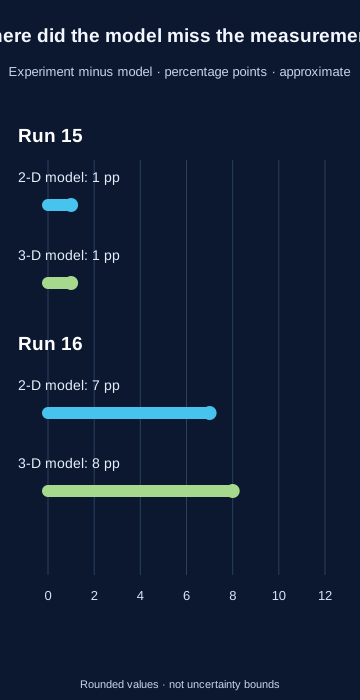
The channel was about half a metre long and 2.03 cm wide. For the two runs discussed, the paper lists a 0.92 T applied magnetic field, hot equilibrium-air conditions with a 5,560 K nozzle-entry total temperature, and electrical conductivities of 130 and 140 mho/m. Its modeled flow was turbulent with a constant ratio of specific heats of 1.25; the experiment maintained steady flow for only about 1.2 milliseconds. The paper says velocity was inferred from flow-generated voltage at the final unpowered electrode pair, which averages the velocity profile.
For Run 15, the paper reports about 27% measured velocity increase and about 26% in both its 2-D and 3-D calculations. For Run 16, it reports about 38% measured, compared with about 31% and 30% in the 2-D and 3-D calculations. These are approximate source-reported comparisons without uncertainty bars; they are not a new measurement by this project. The electric and magnetic fields act on an accelerator channel. This paper does not establish a generator powering that accelerator, a closed vehicle energy budget, net aircraft thrust or flight performance. NASA NTRS record: Kato et al., AIAA 2004-0317 · Full NASA-hosted conference paper. The paper cites the earlier channel experiment reports NASA TM-2001-210922 and AIAA 2003-4285; consult those primary experiment reports before any standalone reanalysis.
A defensible cycle needs one declared configuration and operating point: inlet capture area and mass flow; bleed and fuel addition; station-by-station pressure, temperature and velocity; generator extraction and pressure loss; electrical output and field/auxiliary loads; heat transfer and cooling; combustion; accelerator work; nozzle exit area and pressure; and external drag. Measurements or cited model inputs must share those same conditions. Until then, these separate results show useful component evidence and questions to test—not a demonstrated net thrust benefit.
This comparison follows the stated limits in the NASA Mach 6 inlet report, the AFRL HVEPS summary, and the NASA MHD-cycle analysis. These sources describe different experiments and model boundaries.
Simple version: Researchers planned to send very hot gas through a short channel with magnets and electrodes, then measure how its speed and temperature changed. A plan explains what they intended to test; it is not proof that the planned test succeeded.
The 2001 preprint describes the EAST shock tunnel and an MHD accelerator channel that was still being fabricated. It gives the accelerator length as 23.7 cm and a 20–30% velocity increase at 3.5–4 T as an idealized one-dimensional analysis estimate, not a measured result. These planned conditions must not be combined with the separate NASA Ames 2004 channel runs shown below.

This early test plan gives context for how the apparatus was intended to work. The published 2004 experiments are a later, separate source record; neither source demonstrates a generator-powered aircraft loop or whole-vehicle net thrust.
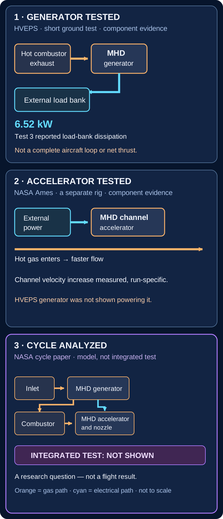
Simple version: One experiment made electricity from hot gas. A different experiment used electricity to speed up hot gas. A computer study connected the ideas on paper. Those are three separate kinds of evidence.
The NASA cycle model also includes a diffuser, power conditioning and a pre-ionizer; this simplified drawing focuses on the generator-to-accelerator energy path. The cited component tests do not demonstrate that modeled engine as integrated hardware.
| Panel | Source evidence | What it does not establish |
|---|---|---|
| HVEPS generator | Mach-8-simulating short ground test; Test 3 reports 6.52 kW load-bank dissipation. AFRL program account · Lineberry et al., AIAA 2007-3880 | Not an aircraft power bus, an accelerator powered by the generator, or net thrust. |
| NASA Ames accelerator | Separate externally powered channel tests reported increased averaged flow velocity. Kato et al., NASA NTRS 20040105526 | Not a generator-to-accelerator loop or an aircraft thrust measurement. |
| NASA cycle | Published thermodynamic cycle analysis of a generic diffuser–generator–combustor–accelerator–nozzle configuration with power conditioning and a pre-ionizer. NASA NTRS 20000095934 | This cycle calculation is not an integrated hardware test, flight demonstration or proof of net vehicle benefit. |
Simple version: Imagine a fast ball slowing down. Its motion energy changes form; a nearby wire does not automatically catch that energy as electricity. In this ideal inlet model, the air's motion energy becomes a change in the air's pressure-and-temperature energy. No electrical energy is produced.
At the model's default Mach 5 inlet and Mach 2 outlet, 515.7 kJ per kilogram is the calculated decrease in flow kinetic energy. The model gives an equal increase in static enthalpy and keeps total enthalpy constant. It is an energy-accounting result for the stated perfect-gas assumptions, not a measured store of electricity or a prediction for an actual vehicle.
A magnetohydrodynamic (MHD) generator is a separate process: a sufficiently electrically conductive gas moving through a magnetic field can produce electrical output. Extracting energy brakes the gas. The conductivity, magnetic-field system, pressure loss, cooling and electrical conversion all affect the complete energy balance. Ordinary passive electrodes in air do not convert the inlet's pressure or temperature rise directly into electricity.
A short-duration ground test ran a scramjet combustor with an MHD generator installed downstream in hot exhaust at simulated Mach-8 conditions. The public reports give figures with different levels of detail and access; keep each number attached to its own source.
| Source | Reported output | What the available report establishes |
|---|---|---|
| AFRL program summary | 2–10 kW | The official AFRL account reports a Mach-8-simulating ground test and 2-10 kW output, and states that output was limited only by the test rig's mass-flow rate. The account gives no point-by-point data or explicit metering boundary; do not combine this range with separate participant peak reports. |
| General Atomics participant account | 15 kW preliminary peak | The account describes a peak over the generator’s active section; it is not whole-engine net power. |
| Lineberry et al., AIAA 2007-3880 | Abstract: 14.8 kW peak; body Table VI: 6.52 kW measured at the load bank, 14.38 kW post-test active-channel estimate, and 14.80 kW calculated at matched load for Test 3. | The full 32-page preprint is now inspected. The abstract's 14.8-kW wording is broader than the body-table classification; Table VI's notes identify the 14.80-kW matched-load value as post-test analysis, not the measured load-bank point. |
The retained 32-page AFRL preprint copy provides useful boundary detail: for Test 3, 6.52 kW was dissipated at the load bank, 14.38 kW is a post-test active-channel estimate excluding end losses, and 14.80 kW is the calculated matched-load maximum. The paper abstract describes 14.8 kW as a peak electric output, but its Table VI and notes classify the 14.80-kW value as analysis rather than the measured load-bank point. General Atomics separately reports a preliminary 15-kW peak over the active section; closeness in scale does not prove identical processing or measurement boundary. AFRL's 2-10-kW summary range is compatible in scale with load-bank readings across the listed tests, but does not identify a matching output definition. Its separate summary phrase that output was “limited only” by rig mass flow is summary wording for that demonstration, not a general scaling law: the detailed report discusses combustion efficiency, plasma and ionization conditions, possible seeding variation, and electrical losses; it also states that NaK seed flow was not directly measured (Table VI, printed p. 27 / PDF p. 29; discussion, printed p. 29 / PDF p. 31). These caveats do not establish a vehicle-level power or thrust benefit. AFRL summary · official report record. The 2008 journal analysis of HVEPS Run 3 discusses measured load current and voltage and voltage differences along the channel; it does not close vehicle-bus power or provide a complete uncertainty budget. Retained third-party indexed preprint copy; selected Table VI rows checked against the official NTIS/NTRL PDF | Ishikawa et al. (2008), pp. 1444-47. These are short-duration ground-test generator results, not flight performance or an inlet-to-generator-to-accelerator demonstration.
Simple version: The paper draws two lines for electricity sent to a resistor. It explains how the fast DAQ power trace was made. It says the Fluke backup meter recorded terminal voltage, but does not explain how that second line was converted to power. So that line cannot be an independent power check. The report links “Run 3” to Test No. 3 (UTRC 213.3); the plotted readings are not the original data file.
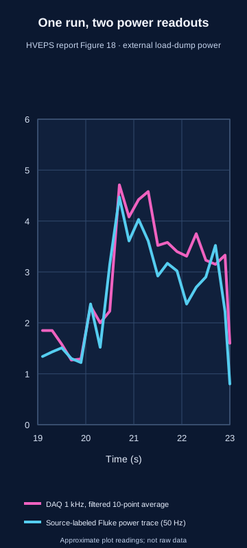
Simple version: Power tells us how fast energy moves. Add the little slices under a power-versus-time line and we estimate energy. Across the 3.9 seconds sampled (19.1 to the 23.0-second plot edge), the DAQ curve suggests about 11.6 kJ dissipated in the resistor. The Fluke-labeled curve would imply about 10.3 kJ only if its plotted values are power; the report does not document that calculation. This window is not shown to match the test's nominal three-second power interval.
| Source trace | Conditional energy estimate over 19.1–23.0 s | Amplitude-only sensitivity | Exact base-12 form of graph-read rational |
|---|---|---|---|
| Filtered 1 kHz DAQ, 21 plotted samples | about 11.6 kJ (unrounded calculation: 11.6205 kJ) | 10.8405–12.4005 kJ | B.7542830A44BAA214165225B5…₁₂ |
| Source-labeled 50 Hz Fluke curve, 21 graph-read samples | about 10.3 kJ (unrounded calculation: 10.271 kJ) | 9.491–11.051 kJ | A.3303557B7485461889B98428…₁₂ |
Method: composite trapezoidal integration of the graph-read samples; 1 kW·s = 1 kJ. The first 0.1 s after the plot's 19 s boundary is unsampled and excluded; the final point sits at the 23 s plot edge. The sensitivity column shifts every ordinate together by ±0.2 kW across the 3.9 s sampled span. It is only an amplitude sensitivity check: not a confidence interval, not a complete uncertainty bound, and not instrument uncertainty. The source labels both curves as external load-dump power, but does not document the Fluke curve’s power calculation or current pairing. Do not treat it as an independent power measurement, or add or average the curves. This is energy dissipated in a ground-test resistor, not energy recovered for a vehicle bus. Table VI separately reports 6.52 kW for Test No. 3; its 57.82 A and 1.95 ohm give 6.519 kW by I-squared-R, consistent with that rounded table value. Figure 18's graph ends at 6 kW, so it cannot verify 6.52 kW exactly. The paper says its post-test analysis averaged 100 filtered 1 kHz samples from a subjectively chosen maximum-power region, while this integral covers 3.9 plotted seconds. The paper does not publish exact sample indices or tie Figure 18's 19-23 s axis to Table IV's nominal three-second power-generation hold. These are related views of the same test, but not a reconciled power history or a measured three-second energy total. The report crosswalks Run 3 to Test No. 3 (UTRC 213.3) through Table V and Figure 27; the plot still supplies no raw DAQ file or calibration package. Figure 18 spans 0–6 kW, so its graph-read trace cannot verify Table VI's 6.52 kW exactly. Table VI's 57.82 A and 1.95 ohm are internally consistent with 6.519 kW by I-squared-R. The report says 100 filtered 1 kHz samples from a subjectively selected maximum-power region were averaged for post-test analysis, but does not publish their indices. Its Figure 18 19–23 s axis is not linked to Table IV's nominal three-second hold; this 3.9-second integral is not an exact reconciliation or measured three-second energy total. Base-12 digits are exact conversions of the decimal graph-read rationals (DAQ 23241/2000 kJ; Fluke 10271/1000 kJ); they encode the same approximate readings and add no physical precision. Integrated values and sensitivity method · CSV · Full digitization and integration methods · JSON.
What the original report labels: Figure 16 contains raw terminal voltage and current traces explicitly identified as Test No. 1. Figure 18 contains load-dump power labelled Run 3, not a raw voltage/current pair; Table V maps Test No. 3 to UTRC 213.3 and Figure 27 explicitly labels the Run 3 model/data set as Test No. 3. Do not use Figure 18 to claim a reconstructed Test 3 trace or a complete power balance. A separate indexed extract attributed to AFRL-PR-WP-TP-2007-232 mixed in a voltage/current Figure 2 caption, but that report number belongs to Thibodeaux's distinct space-charge study (ADA473277, AIAA 2007-4518); the official HVEPS report is AFRL-PR-WP-TP-2007-233 (ADA471429), whose Figure 2 is a combustor-rig schematic. Official NTIS/NTRL record for the separate 2007-232 report · Thibodeaux AIAA 2007-4518 metadata · HVEPS test-results paper, AIAA 2007-3880. Some secondary citations show 3881; DOI registration supports 3880.
Simple version: A generator can take some electricity from hot, moving gas. But the whole engine only helps if its returned benefit is worth the extra power, heat, pressure loss and equipment needed to make it work.
What the official HVEPS report says: its best reported test separates three different quantities. Test 3 has 6.52 kW reported load-bank dissipation (reduced from recorded electrical channels; consistent with the listed 57.82 A and 1.95 Ω via I²R ≈ 6.52 kW); a post-test analysis estimated 14.38 kW across the active channel after excluding end-region losses; and Table VI gives 14.80 kW at a matched load, its maximum for the 89.0% mean-combustion case. At 81.5% and 96.5% combustion efficiency, its low/high analyses give 15.98 and 15.19 kW, respectively. All three matched-load figures are post-test calculations, not measured load-bank outputs; 14.80 kW should not be described as the directly measured load-bank output. The abstract calls 14.8 kW an electric-output peak, but Table VI and its notes place 14.80 kW in the calculated matched-load column. The 15-kW participant summary is close to the active-channel estimate, but exact run and meter equivalence is not stated. AFRL's broad 2–10-kW range is compatible in scale with measured load-bank outputs across the listed runs; the public summary does not confirm that this is precisely the same quantity.

| Value | Quantity | Evidence type |
|---|---|---|
| 6.52 kW | Power dissipated at the external load bank | Reported load-bank dissipation, reduced from electrical channels; Table VI lists 57.82 A and 1.95 Ω (I²R ≈ 6.52 kW) |
| 14.38 kW | Output across the active generator portion, excluding end-region losses | Post-test derived quantity reported in Table VI |
| 14.80 kW | Maximum output at a matched load | Post-test load-line model estimate, not the measured load-bank point |
The report gives six reduced test points, not a single general-purpose power number. For each point, the load-bank column is the power dissipated at the actual selected resistance; the active-channel column excludes end-region losses; and the matched-load column is a post-test calculation. The bars keep those categories separate.

| Test | Peak field (T) | Combustion efficiency | Load-bank dissipation (kW), reported measured point | Active-channel power (kW), end losses excluded | Matched-load maximum (kW), post-test analysis |
|---|---|---|---|---|---|
| 1 | 1.48 | 91.0% | 3.81 | 6.55 | 8.24 |
| 2 | 1.48 | 85.0% | 3.20 | 4.00 | 7.76 |
| 3 | 1.48 | 89.0% mean case | 6.52 | 14.38 | 14.80 |
| 5 | 1.80 | 81.5% | 5.55 | 7.25 | 8.09 |
| 6 | 1.80 | 77.0% | 5.83 | 8.46 | 8.48 |
| 7 | 1.80 | 82.0% | 2.10 | 2.98 | 6.94 |
The paper reports seven powered tests, but Test 4 is missing from the reduced results because its scramjet pressure distribution was anomalous. It also reports three combustion-efficiency cases for Test 3; this display uses the mean case and leaves the low/high matched-load calculations in the caption. These are rig-level generator results under brief ground-test conditions. None is power returned to a propulsion accelerator or net aircraft power.
The paper also says unregulated end regions reversed the Hall field and caused losses; the authors estimated roughly 25–60% end-region loss. This is a real engineering lesson about where power is measured and how a generator is loaded, not evidence of an aircraft-level net gain. The test lasted only seconds under ground-facility conditions; the electrical load was a resistive bank, and no accelerator loop, installed-system mass or vehicle thrust benefit was tested. Retained third-party indexed preprint copy; selected Table VI rows checked against the official NTIS/NTRL PDF · AIAA conference-paper record · General Atomics participant summary.
Simple version: HVEPS measured electricity from one generator on a ground rig. To know whether a whole aircraft could gain energy, researchers would also need matching air, fuel and seed flows, all the power used to run the equipment, heat and pressure losses, and thrust. The report does not give all of these together for the same moment. Its flow numbers have different statuses: Table II contains calculated target points; Table III lists the MHD-test set conditions and, separately, a March 2006 unseeded baseline. Neither table gives species flow synchronized to Test 3’s selected power samples. Lineberry et al. (2007), Tables II–III (printed pp. 9 and 11; inspected in the retained preprint).

Simple version: The generator switches on, produces electricity briefly, then winds down. The first graph keeps the fast wiggles in the recorded voltage and current; the second smooths the same run so the broad changes are easier to follow.
The report identifies these as HVEPS MHD Test 1, Figures 16 and 17. Figure 16 shows terminal voltage and net load current recorded at 1 kHz from about 27 to 35 seconds. The authors place seed injection near 27.68 s and the main generation interval at about 3 s, ending near 30.7 s. They attribute the current spike near 32.2 s to purging the NaK feed while the slower ethylene shutoff briefly left combustion and seeding overlapping. They describe slower signal variation as combustion unsteadiness and faster fluctuations as electrical arcing in the channel.
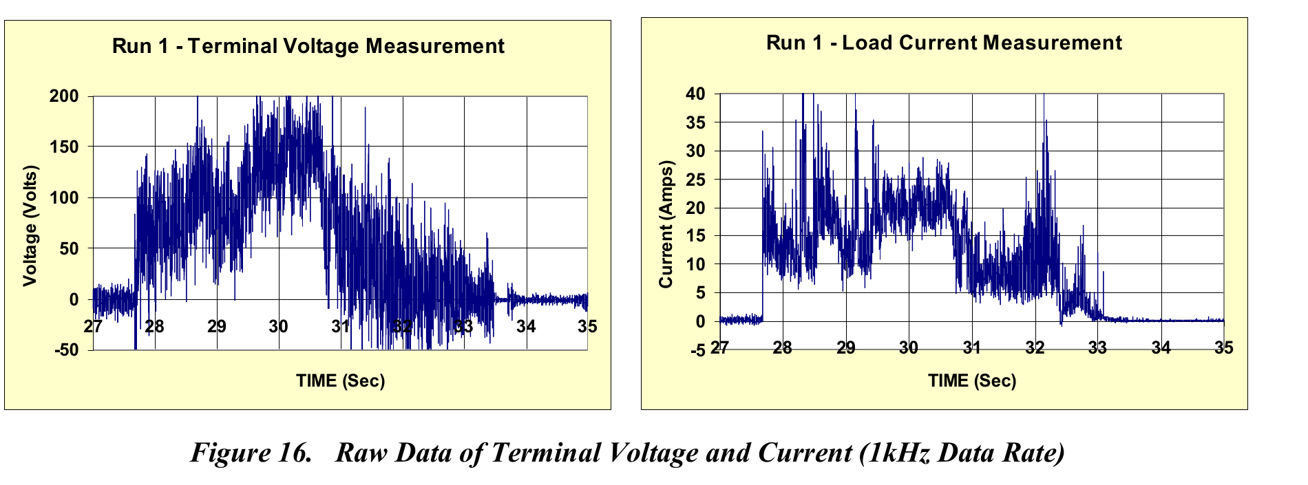
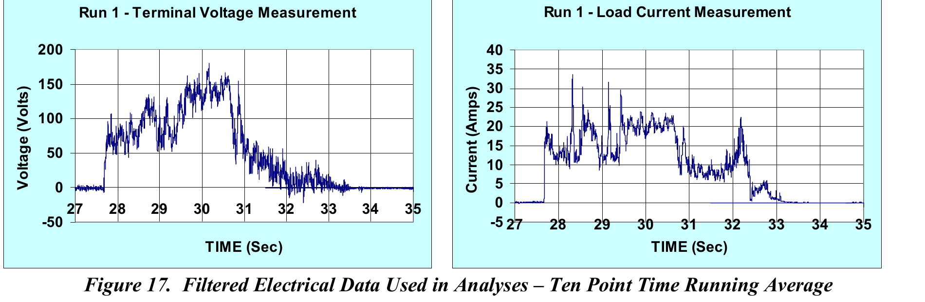
What this does not establish: These are Test 1 images, not Test 3 samples behind the 6.52 kW load-bank result. A ten-point filter suppresses fast variation and changes the displayed waveform. The retained report copy supplies plotted traces, not machine-readable samples with a full calibration and uncertainty record; these images alone do not support a precise time-integrated energy estimate. No synchronized complete-loop input/output or vehicle-thrust benefit was demonstrated.
| Quantity | What the report gives | What remains open |
|---|---|---|
| Load-bank electricity | Reported load-bank dissipation: 6.52 kW; Table VI lists 57.82 A at 1.95 Ω. I²R gives 6.519 kW, consistent with rounding. Figures 16–18 show recorded electrical traces, including a plotted 1 kHz Test 1 voltage/current trace. | No machine-readable synchronized Test 3 samples, calibration certificates, or complete electrical uncertainty budget were found in the retained report/source search. The plotted Test 1 trace is not a Test 3 data file. |
| Generator-channel power | 14.38 kW post-test active-channel estimate; 14.80 kW calculated maximum at matched load. | These are not the measured load-bank operating point. |
| NaK seed flow | The setup and intended feed are described. | The authors say NaK flow was not directly measured; its actual run-by-run rate is unknown. |
| Air and reactant flow | Tables II–III contain target, demonstration-series set-condition and separate baseline flow records, summarized in the figure above and transcribed in the downloadable ledger. | No species-flow record is synchronized to the selected Test 3 electrical samples. Do not use the target or baseline flows to calculate kJ/kg from those kW values. |
| Uncertainty | Table VI gives ±7.5% accuracy for combustion-efficiency calorimetry. | That is not an uncertainty estimate for electrical output; meter and propagated uncertainties remain open. |
| Support power and heat | The report describes the magnet, seed system, heat-sink channel, and purge/cooling sequence. | A synchronized total of magnet, conditioning, controls, seed, cooling, and rejected-heat terms on one boundary. |
| Accelerator and vehicle force | No accelerator or thrust value is reported for this HVEPS test. | A matched generator-to-accelerator run, nozzle force, installation losses, and vehicle comparison. |
This ledger is limited to the inspected report; “not reported here” does not prove that no additional records exist. The test establishes a short-duration ground generator result, not a closed energy loop or aircraft benefit. Retained third-party indexed preprint copy; selected Table VI rows checked against the official NTIS/NTRL PDF · AIAA paper record · Source-to-claim ledger · JSON · Open questions · CSV · Rebuild the CSV · Python.
Simple version: Researchers measured how much current came out of the generator. A computer model then tried to reproduce that pattern. It matched the middle of the generator well, but the model and measurements differed near the two ends.
Ishikawa and colleagues’ 2008 open journal paper analyzes the experimental HVEPS Run 3 conditions and results described in Lineberry et al. (2007). It is a numerical re-analysis of that ground test, not a new experiment or a source of synchronized raw telemetry. The paper compares the calculated load current with the measured current across the channel.

| Insulator number | 3D model current · graph read | Measured current · graph read |
|---|---|---|
| 3 | ≈42 A | ≈58 A |
| 5 | ≈60 A | ≈58 A |
| 7 | ≈73 A | ≈58 A |
| 8 | ≈76 A | ≈58 A |
| 9 | ≈77 A | ≈58 A |
| 10 | ≈72 A | ≈58 A |
| 12 | ≈65 A | ≈58 A |
| 14 | ≈61 A | ≈58 A |
| 16 | ≈59 A | ≈58 A |
| 18 | ≈58 A | ≈58 A |
| 20 | ≈59 A | ≈58 A |
| 22 | ≈58 A | ≈58 A |
| 24 | ≈59 A | ≈58 A |
| 26 | ≈61 A | ≈58 A |
| 28 | ≈66 A | ≈58 A |
| 30 | ≈72 A | ≈58 A |
| 31 | ≈71 A | ≈58 A |
| 32 | ≈68 A | ≈58 A |
| 34 | ≈61 A | ≈58 A |
How the model was set up: The paper describes a fully coupled three-dimensional fluid and electrical calculation: time-dependent compressible flow equations, steady Maxwell equations under the MHD approximation, and thermochemical-equilibrium properties. For Run 3 it used inlet pressure 0.284 atm, inlet temperature 2,480 K, Mach 2.02, a 1,000 K wall and peak magnetic field 1.48 T. Its computed pressure-based MHD interaction parameter was 0.0034, so the authors expected only a small change to the flow field.
A fitted input, not an independent validation: The ideal thermochemical calculation predicted too much current. The researchers multiplied ideal scalar conductivity by δ = σ/σideal = 0.813 to bring modeled current closer to measurements in the active channel. That means 81.3% of the ideal value was retained—a reduction of about 18.7%, not a loss of 81.3%. The authors said the cause was unclear and suggested incomplete combustion and non-uniform mixing, seed distribution or temperature as possible contributors. Because δ was adjusted against the same measurements, the resulting agreement is a calibration-like comparison, not independent validation.
Losses and limits: The calculation produced about 100 V total electrode voltage drop, roughly 30% of its modeled induced voltage in the active region. These values depend partly on its arcing model and imposed 1,000 K wall temperature. The grid had 128 × 41 × 21 cells; the paper says about 0.2 mm cells would be needed to resolve a near-wall arc scale around 1 mm, so its grid was coarse for that feature. It identifies eddy-like currents in the end PTO regions but says more detailed electrodynamics are needed to quantify their power-loss effect. The article does not close auxiliary loads, whole-vehicle energy, net thrust or an aircraft benefit.
Reference-number note: Ishikawa et al. cite their Run 3 experimental source as AIAA-2007-3881 (their Reference 3), while the DOI record and other project records identify the HVEPS test-results paper as AIAA 2007-3880. This numbering mismatch is unresolved; we preserve what each source says rather than silently correcting it. The underlying report record is AFRL/NTIS-NTRL ADA471429.
Ishikawa et al. (2008), full paper, Figures 4–11 and conclusions, pp. 1444–47 · AIAA 2007-3880 DOI record (numbering discrepancy above). Local retained PDF SHA-256: E903DFB069B9A8C600646A1DD45DA59D911327BB8F863A88DEB01C0CBDA4E7B7.
Simple version: Researchers ran hot combustion gas through a small magnetic generator, recorded electrical, pressure and thermal data at several channel locations, and compared the results with a computer model. This shows what one generator component did and how its model compared with the measurements.
Keep the experiments separate: the 2008 UTSI annual report describes eight combustion-driven tests in the UTSI Propulsion Laboratory, using a separate combustor, a Hall MHD channel and a superconducting magnet. The AIAA paper identifies the demonstration firings as August 2007. This is not the December 2006 UTRC scramjet-driven air/seed test described in the adjacent HVEPS evidence: the facilities, flow arrangements and reported measurements differ, even though both sit within the wider HVEPS program.
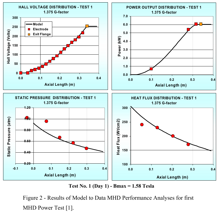
What it establishes: component-level MHD generation and measured-versus-modelled electrical and thermal distributions in this UTSI setup. The report calls the plotted power a distribution of internal power developed along the channel; it is not a whole-engine surplus. Do not merge it with the separate UTRC Test 3 load-bank value of 6.52 kW, and do not infer an accelerator benefit, vehicle thrust, or closed system efficiency. Neither HVEPS campaign supplies a synchronized whole-vehicle energy-and-force balance.
A separate NASA hot-gas experiment in 1980 measured gross electrical output from a cesium-seeded hydrogen–oxygen combustion stream. The nominal conditions were 10 atm combustion pressure, 0.5 kg/s mass flow, 7 MW thermal input and a peak magnetic field of 5 T. Two Hall-duct configurations reached reported maximum outputs of 87.5 kW and 153 kW at the generator load. Dividing those outputs by the stated thermal input gives 1.25% and 2.19%, respectively. This transparent output-to-input comparison is not net plant efficiency: the report does not close the magnet, cooling, seed, pump and other facility loads, and electricity was not returned to a propulsion accelerator. The 58 cm duct ran in pulsed tests; data runs lasted five seconds, and its exhaust was water-quenched at atmospheric pressure. NASA-TM-81424 record · Download the 19-page NASA report (PDF).

Simple version: The team made and measured electricity from hot gas for a few seconds. That proved the generator component could work in this test rig. It did not show that a whole engine would gain useful power after magnets, cooling, pumps and other equipment were counted.
| Question | What the report says | What remains unshown |
|---|---|---|
| What was tested? | A cesium-seeded hydrogen–oxygen combustor fed a Mach-2 Hall generator in a cryomagnet; nominal conditions included 10 atm, 0.5 kg/s, 7 MW thermal input, 5 T peak field and a 58 cm duct (printed pp. 2–4). | This is a laboratory combustion-gas generator. No flight engine or propulsion accelerator was powered by its output. |
| How long and where did the exhaust go? | The reported data runs lasted 5 seconds; high-field operation was pulsed. The duct exhaust was water-quenched, with the flow discharged at atmospheric pressure (printed pp. 2–4, 8). | The proposed H₂/O₂ topping-plant case needed very low sub-atmospheric exhaust pressure. NASA says generator performance there was not established. |
| What constrained output? | For the 4:1 area-ratio duct, a shock appeared at about 7 atm and below even with no power extraction; stronger field moved the shock upstream and changed the output trend. In separate open-circuit tests, breakdown occurred above about 50 V per insulator after roughly 2.5 seconds of seed injection; damage was found on anode-side insulators (printed pp. 6–7). | These limits are specific to the reported ducts and conditions. They warn that stronger magnetic field does not guarantee proportionally more usable power. |
| Was large-scale cycle performance demonstrated? | The report says an attractive proposed topping plant required roughly 40% enthalpy extraction and that very large facilities and vacuum testing would be needed (printed pp. 6–8). | The report explicitly leaves this extraction level and low-pressure performance as open questions. Its 87.5 and 153 kW values are generator outputs, not proof of net plant efficiency. |
Source: J. Marlin Smith, Experiments on H₂-O₂ MHD Power Generation, NASA-TM-81424 (1980), printed pp. 2–8. NASA report record · NASA-hosted PDF.
The plotted ratios use the report’s numbers: 87.5 kW ÷ 7,000 kW = 0.0125 in decimal, which is 0.01(9724) in base 12 (digits 9724 repeat). The operands are 73.6₁₂ kW and 4074₁₂ kW. For the second duct, 153 ÷ 7,000 = C9₁₂ ÷ 4074₁₂ = 0.021857… in decimal, reported as 2.19% after rounding. Base 12 changes the notation; it does not change the measurements, uncertainty or efficiency boundary.
Conditions, evidence categories, source hash and arithmetic · JSON
Simple version: Hot gas does not always let electricity move through it. Before the test, the team used calculations to see how adding oxygen might change whether this hot gas could carry electricity. This helped choose test conditions; it was not a result from the generator test.
The published Figure 11 plots design-level estimates for conductivity and diagonal MHD power density. Its curves are model calculations, not experimental measurements. This original redraw uses approximate readings from the published raster plot; no pointwise numerical file is provided. Dots mark estimated source points, and connecting lines are visual guides only.
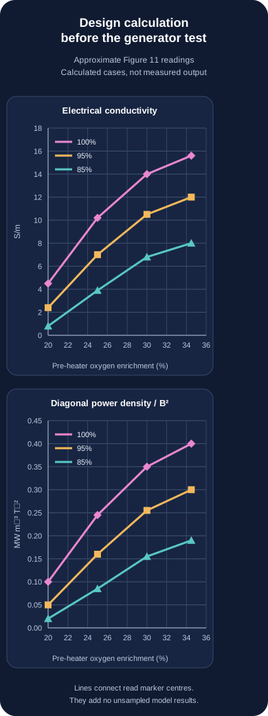
Keep the two power-density quantities separate. Table II lists 8.06 S/m and 7.81 MW·m⁻³·T⁻² for its 85% target at 35% oxygen enrichment; 7.81 is a Faraday parameter. Figure 11 instead plots diagonal power density normalized by magnetic-field squared, about 0.19 near the 34.5%, 85% design point. These definitions differ, so the values are not a contradiction or direct comparison. The report says RASCAL and LyTec thermochemical codes produced the design calculations; their solver inputs and pointwise output are not available here. A separate, unseeded March 2006 baseline measured 84% mean combustion efficiency, but that does not make these curves measurements.
This calculation helped researchers choose conditions for a hot-flow generator test. If future tests show that useful electricity can be recovered after all losses are counted, this research could help engineers study energy use in very fast aircraft. Figure 11 itself does not show electrical output, net energy recovery, a generator-to-accelerator loop or flight performance. Official NTIS/NTRL ADA471429 report · Wide graph · Phone graph · Approximate readings · CSV · Methods and limits · JSON · Rebuild · Python
Simple version: A computer study can give us a useful map, but it is still a map. One 2024 study modelled electricity generation inside one scramjet MHD channel. Its abstract reports that the generator efficiency stays near 22%, while the channel takes less than 0.35% of the hot flow’s enthalpy in the listed cases. That means the model predicts converting a small slice of the flow’s energy, even if the generator converts part of that slice to electricity. The abstract does not define exactly what each percentage is divided by, so neither number tells us the useful net energy for a whole aircraft. Do not read either curve as whole-engine or net efficiency.

| Magnetic field (T) | Generation efficiency reported (%) | Enthalpy-extraction rate reported (%) | Evidence type |
|---|---|---|---|
| 1 | 22.5 | 0.026 | Simulation, as reported in abstract |
| 2 | 22.3 | 0.10 | Simulation, as reported in abstract |
| 3 | 22.0 | 0.21 | Simulation, as reported in abstract |
| 4 | 21.5 | 0.34 | Simulation, as reported in abstract |
A separate 2025 study adds a mathematical MHD generator after the scramjet combustor. Its baseline engine model was compared with one Mach-7 test point, with reported isolator errors of 2% in Mach number, 4.65% in static temperature, and 17.28% in static pressure. The added MHD channel was compared with a CFD simulation for one channel condition, not with an experiment of an operating MHD generator. For a 2.5 T magnetic field and load factor 0.4, the paper predicts a 3.58% specific-impulse penalty at 0.5% enthalpy extraction and 6.43% at 0.9%. These are model outputs for post-combustor energy extraction; they are not measured thrust losses and do not test an electricity-return loop. I reviewed selected publisher-indexed PDF text; the publisher blocked direct PDF retrieval, so a full visual page-by-page check remains open. Liu, Wu & Meng (2025), Journal of Propulsion Technology · Official article record · Publisher PDF.
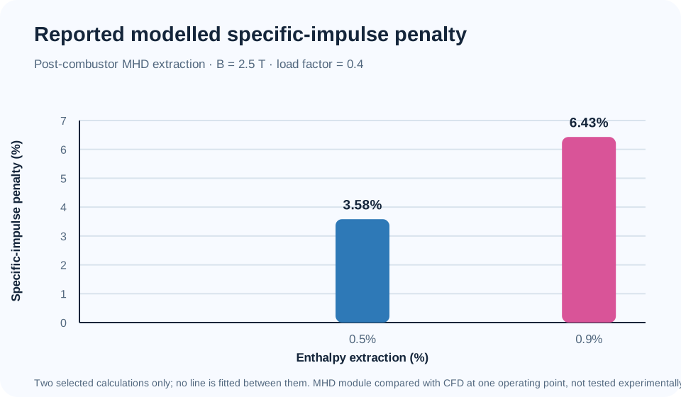
Simple version: A powerful magnet can guide forces on an electrically conducting gas, but the magnet does not supply the energy. In an aircraft concept, energy would come from the moving air and the system would have to overcome electrical, heat and pressure losses. In a space rocket, the spacecraft instead carries propellant and electrical power. These are different engines with different energy accounts.
Lieu’s paper, available online on 6 September 2026 as an in-press journal pre-proof, presents a reduced-order model for both cases. Its abstract describes the aircraft case as a hypersonic MHD thrust augmentor in which ionized shock-layer or boundary-layer gas helps make a larger captured air stream conductive. For one representative Mach 7, 30 km, 0.5 m² scenario, the model estimates a 5 kN thrust increment would require about 11 MW of ideal power removed from the flow and plausibly tens of megawatts of electrical power after losses. These are author-reported screening estimates, not measured performance.
The paper’s space case is separate: it accelerates onboard propellant with a plasma device. The paper therefore does not show that the atmospheric 516 kJ/kg ideal inlet energy can be converted into usable electricity, that a complete aircraft energy loop closes, or that an MHD system has flown. We checked the publisher metadata, abstract and indexed highlights; the full text was not independently reviewed here. Lieu (2026), Aerospace Science and Technology, article 113752, DOI 10.1016/j.ast.2026.113752 · Publisher record and abstract.
Simple version: To make a gas generate electricity, it must carry electric current. One proposed way to help was to keep the gas ionized with an outside power source. A NASA model from 2001 found that, in one example, this ionizer needed much more power than the generator made.
In that modeled case, the ionizer demand was about 827 MW, while the MHD generator produced about 151 MW—roughly 5.48 times as much input as gross generator output. Their simple arithmetic difference is 676 MW (827 MW minus 151 MW): the listed ionizer demand is that much greater than the listed gross generation. This subtraction compares only those two rounded model values; it is not net aircraft power or a complete vehicle power balance. The authors assumed a 100%-efficient ionizer, an optimistic idealization, and reported a modeled case rather than a hardware test. The same table reports the ionizer demand as about 85% of the modeled hydrogen fuel-energy rate, using complete combustion at room temperature. This ratio compares the two listed electrical powers only; it is not a complete vehicle power balance. It does not prove that every MHD design fails. It shows why any proposed design must count ionization and other support loads alongside the electricity it generates. NASA record · Conference paper PDF (Table 1, printed pp. 5–6; conclusions, p. 7).

Simple version: One paper reports a ground test; another describes a computer study. A computer study can help explain a test, but it is not another test. We have not found enough open model files to check whether the computer study reproduces the experiment.
| Publication | Evidence type | What is available here | What it does not establish |
|---|---|---|---|
| Lineberry et al. (2007), AIAA 2007-3880 / AFRL preprint ADA471429 | Hot-gas ground test of a generator component | The retained report copy gives reduced Table VI values. Its PDF hash and locators are in the downloadable input ledger. | An official copy was retrieved through the NTIS/NTRL ADA471429 record (32 pages; SHA-256 CCBC90C0BC0626328B058023D153D2F268767F85DAFD8BFD2A0DBFFACCFA1521). Its hash differs from the retained third-party file. Side-by-side comparison of Table VI (printed p. 27 / PDF p. 29) confirms the displayed rows, including Test 3 low, mean and high load-line cases. The retained color file remains the basis for existing source-image crops. The official DTIC search reported offline on 2026-10-02; the NTRL route supplied this report copy. Synchronized Test 3 flow/electrical files and a complete electrical calibration package are still absent from this report. Official NTIS/NTRL record and PDF download (ADA471429). |
| Gotoh et al. (2007), AIAA 2007-4015 | Computational analysis associated with HVEPS | Crossref confirms the paper’s bibliographic record; DOI metadata and source status are linked below. | Full paper, model inputs and machine-readable results were not located in this bounded review. It has not been independently reproduced and cannot be presented as a measurement or as a resolution of the test-data gaps. |
Crossref registers the HVEPS test-results paper as AIAA 2007-3880. Some later bibliographies show “2007-3881”; this is treated as a likely miscitation, not a proven universal correction. Bibliographic details, copy hash and access limits: HVEPS publication and provenance record · JSON · Run-level input ledger · JSON. The official DTIC site reported its public reports search offline on the date above; this does not show that no official copy exists.
These recent studies sharpen the question for future research: what does an MHD stage contribute after its extraction, field, ionization, cooling, pressure-loss and mass costs are all counted against the same engine baseline? Their published models do not settle that full comparison.
NASA’s MAPX work describes a different, externally powered accelerator facility: a 1.5-MWe arc heater drives a 2-MWe MHD accelerator inside a 2 T magnet. Those are facility component ratings, not measured net power returned by an aircraft. The NASA report states that a meaningful fuel-fraction improvement would require electrical augmentation power to exceed the unaugmented source’s thermal power, and calls the onboard power-density challenge daunting. Its 2008 status report was still preparing full-up assembly and testing; the ratings do not establish that the propulsion loop achieved that condition. NASA MAPX status record · Full NASA/TP, introduction and conclusions.
One later turbojet-cycle report leaves a reproducibility question. Eq. (2) (printed p. 5 / PDF p. 9) defines extracted power using mass flow, Cp and generator-inlet total temperature. Using an explicitly chosen heat-capacity range of 1.0-1.2 kJ/(kg K), the Mach 4.75 and 5.25 values in the report's prose imply about 5.9-8.3 MW, while a 76-point digitization of Figure 5 (printed p. 8 / PDF p. 12) reads about 69.9 and 87.7 MW. The 1.0-1.2 range is our sensitivity assumption; NASA does not give its numeric Cp or pointwise NPSS inputs in the inspected report record. A reverse calculation offers another clue: pairing the report's approximate prose endpoints at Mach 4.75, 5.25, 6.00 and 6.75 with the plotted curve gives implied effective Cp values near 12 kJ/(kg K). That cluster is compatible with a shared scale factor or convention, but approximate endpoint pairings can produce a similar pattern. It does not establish NASA's Cp, exact matched run points, or the cause. The same author's 2013, 239-page Kent State dissertation revisits the NPSS cycle in Chapter 5 (printed pp. 80–102; PDF pp. 102–124). It repeats the 45–90 MW extracted-power range and the Mach 4.75–5.25 prose values in §5.4.2 (printed p. 92 / PDF p. 114), and Figure 5.5 gives the corresponding model plot. Table 5.1 (printed p. 82 / PDF p. 104) lists generic NPSS file types and names, not the study's runnable deck or pointwise output. I found no numerical Cp value in the thesis passages describing the equation, so this follow-up does not resolve the mismatch or provide an independent reproduction. No value is corrected and no source error is alleged. NASA/TM-2011-217136 record · NASA report PDF: Eq. (2), Figure 5 and Mach-point text · Official OhioLINK/Kent State dissertation record · Full dissertation PDF.

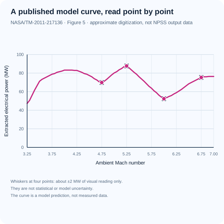
| Ambient Mach | Figure 5 power (MW, approx.) | Prose flow / extraction / temperature | Implied effective Cp (kJ/kg K) |
|---|---|---|---|
| 4.75 | 69.86 | ~10 kg/s - ~50% - 1180 K | 11.841 |
| 5.25 | 87.67 | ~10 kg/s - ~50% - 1380 K | 12.706 |
| 6.00 | 52.40 | ~4 kg/s - ~60% - 1720 K | 12.694 |
| 6.75 | 75.34 | ~5 kg/s - ~60% - 2089 K | 12.022 |
What this tells us: the four implied values average 12.316 kJ/(kg K), but this does not prove a single heat capacity or convention was used. These are approximate statements from the same report, and the last two are analyst-paired trend endpoints, not matched operating-point records. NASA's PDF describes Cp as constant-pressure specific heat but supplies no numeric value, units, property schedule, or NPSS input deck. The apparent scale difference is therefore unresolved. Review the full digitization method and limitations.
Whole-cycle results depend on the configuration and assumptions. The 2000 NASA report includes a full-cycle performance curve; its result is reproduced below as an approximate reading of the published graph because the report provides no numerical point table. Separately, a peer-reviewed 2004 Journal of Propulsion and Power article by Riggins reports that thermally balanced MHD-bypass simulations underperformed the conventional scramjet across the studied Mach 8–12.2 range. Its institutional record currently exposes citation and abstract, not the full paper or numerical curves. This more detailed result and the 2000 simplified cycle have different assumptions and boundaries; do not combine them as one benchmark. Neither establishes flight performance or net vehicle benefit. Riggins (2004), DOI 10.2514/1.4980 · Missouri S&T record and abstract.
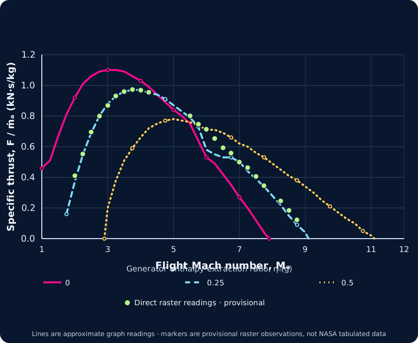
Equation reference note: In the final 2000 report, the Figure 2 discussion points to Eqs. 25 and 28 for the generator and accelerator pressure ratios, but those equation numbers identify diffuser relations in the final equation sequence. By their contents, the component relations are Eqs. 36 and 53. The earlier 1999 NASA preprint used a different numbering: its Eqs. 26 and 30 give the generator and accelerator pressure-ratio relations, and its Figure 2 discussion points to those same numbers. This suggests the final report may retain stale cross-references after renumbering; the reason is not documented. We use the equations by content. This comparison does not verify the digitized curve, our reconstruction, or flight performance. 1999 NASA preprint record · Preprint PDF (Eqs. 26, 30 on PDF p. 8; Figure 2 discussion on p. 11).
The earlier headline comparison against the old line is withdrawn: trace identity was not established, so those discrepancy metrics must not be used. A reproducible project audit records 30 source-raster points: 23 clear and 7 ambiguous. C misses the dashed stroke at separated positions and follows other strokes near Mach 6–7; D also differs on part of the descending limb. These are differences between project graph readings and an analyst-selected raster center trace. They do not measure NASA source/model error; calibration, line thickness, antialiasing, and selection uncertainty are incomplete, and crowded crossings remain ambiguous.
| Approx. Mach | C crop y pixel | Direct dashed-ink y band | Center ordinate from raster (kN·s/kg) |
|---|---|---|---|
| 2.498 | 500 | 400–413 | 0.695 |
| 3.004 | 372 | 287–294 | 0.869 |
| 5.996 | 486 | 389–399 | 0.713 |
| 6.998 | 646 | 531–541 | 0.499 |
Vertical bars show same-column thresholded pixel bands only; horizontal bars show ±0.5 source pixel. Neither is a confidence interval. Axis calibration and curve-selection uncertainty are not fully propagated. Crossing/overlap alternatives and the uncertain endpoint remain in the downloadable project audit. This is an audit of figure readings, not a correction to NASA, flight evidence, or independent reproduction of the cycle calculation.
This independent calculation applies the report's simplified cycle equations. It is not author code, test data, or a vehicle-performance prediction. The calculation uses explicit perfect-air constants and added pressure closures; its ideal ambient-matched nozzle is expanded to ambient pressure separately at every Mach number, so it is not a fixed-nozzle design. Unit pressure ratios are assumed for the pre-ionizer and cooling expansion. The Figure 2 reference case fixes the burner exit at 3000 K while also applying positive energy in the accelerator. The cycle equation therefore necessarily puts accelerator-exit temperature above the report's separate 3000 K accelerator limit for every successful positive-extraction sample. This is a conditional model result, not evidence of tested operation. The dual-cap curve lowers burner temperature to satisfy both constraints; it is a new sensitivity case, not NASA's plotted result.
Simple version: A generator takes some energy from the hot moving air; after a small pre-ionizer share, an accelerator returns some energy to the exhaust. This paper model lets you inspect the temperature and thrust bookkeeping. It is a calculation, not a working aircraft.
Mach values are precomputed at 0.05 intervals from 1 to 12; extraction values are the three cases shown in the report.
Loading the calculated cases…
Specific thrust is normalized per inlet-air mass flow, not total engine force. The model’s pressure-thrust term is zero only because it assumes nozzle exit pressure equals ambient pressure.
Changing a control updates the model explanation and readouts.
The downloadable overlay retains 95 earlier approximate graph readings as an audit history. Its residual statistics describe differences from those project readings; they cannot establish disagreement with NASA's numerical results, and their original graph-reading allowances are not validated total uncertainty.
Why the comparison changed. At flight Mach 6 and generator extraction ratio 0.25, this conditional equation reconstruction gives 0.697 kN·s/kg. The earlier claim of a clear mismatch used an old graph reading of 0.58 ± 0.05 and is withdrawn. A direct raster observation is 0.713 kN·s/kg at its actual calibrated Mach 5.996; evaluating the same model at that Mach gives 0.698, a signed model-minus-reading difference of −0.0155 kN·s/kg. This is a comparison with a manually read image, not NASA-tabulated output. The visible ink band is not total uncertainty, so the comparison establishes neither validated agreement nor a NASA model error. It does not show that NASA’s figure or report is wrong. At exact Mach 6 the reconstructed accelerator-exit stagnation temperature is about 3,418 K. The report states a 3,000 K burner limit for Figure 2 and separately describes the same general temperature limit for the accelerator (NASA PDF pp. 10 and 26); enforcing both requires the distinct dual-cap sensitivity case, not silent reinterpretation of the plotted curve. The energy split itself closes within the model: about 458.84 kJ/kg-air extracted, of which 22.94 is assigned to pre-ionization and 435.90 to the accelerator. These are conditional calculated values, not measurements.
One unresolved reference in the original report: the Figure 2 discussion says the generator and accelerator pressure ratios use Eqs. 25 and 28, but those equation numbers describe diffuser relations; the MHD component pressure-ratio equations are numbered 36 and 53. This reconstruction uses Eqs. 36 and 53 by component definition. The report does not clarify this cross-reference inconsistency. A typo is plausible but unconfirmed; this does not establish that Figure 2 is wrong.
NASA's thrust equation includes both momentum and pressure thrust. The current reconstruction sets exit pressure equal to ambient, which makes the pressure term zero. The report lists a nozzle total-pressure ratio of 0.98, but does not publish the nozzle expansion efficiency or a fixed exit geometry for this plotted case. The graph below therefore sweeps an explicitly chosen exit-pressure ratio, from 0.7 to 1.4 times ambient. It derives the exit area separately at each point from mass continuity, so it is a boundary sensitivity—not a fixed-nozzle prediction and not a fit to NASA's curve. In this conditional calculation, momentum and pressure contributions partly offset one another; the total stays between about 0.694 and 0.697 kN·s/kg-air across this illustrative sweep. The selected range is not specified by NASA, so this does not bound what a real fixed nozzle would do. The reference case also reaches about 3,418 K after the accelerator, above the report's separate 3,000 K limit.
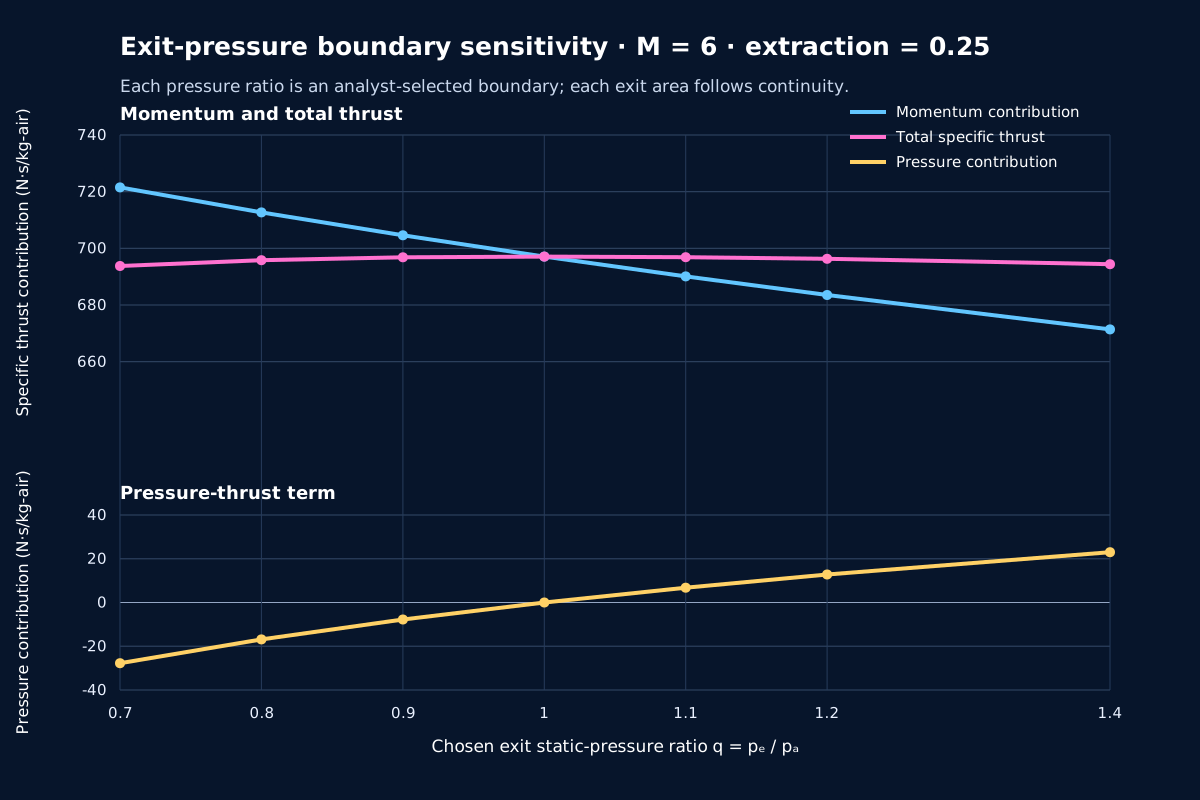
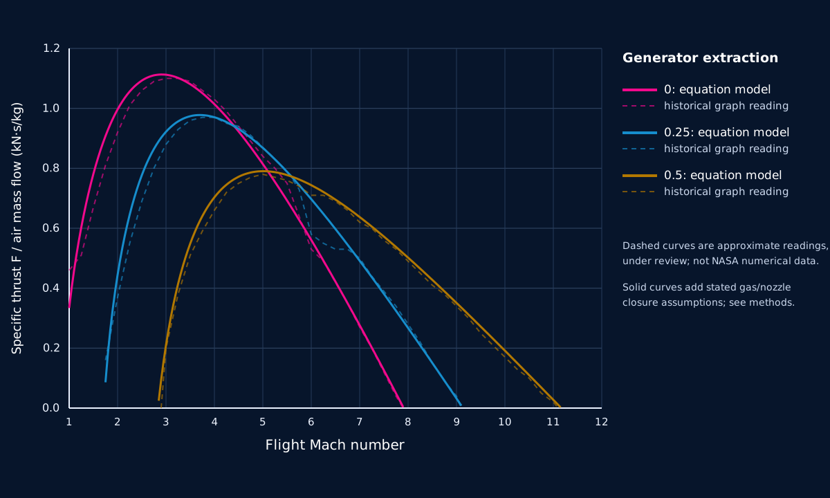
The values are conditional on the paper's simplified cycle. Its authors caution that the assumed component pressure ratios are held constant for simplicity and are not independent of flight Mach; the MHD-device efficiencies are optimistic assumptions, and the pre-ionizer power share is selected only for demonstration.
| Gas and inlet state | Thermally and calorically perfect gas; freestream static temperature 220 K. |
|---|---|
| Fuel and burning | Fuel heating value 45 MJ/kg; assumed combustion efficiency 100%. |
| Pressure ratios | Diffuser 0.70; burner 0.95; nozzle 0.98, held constant for simplicity. |
| MHD devices | Generator and accelerator isentropic efficiencies each assumed to be 0.90. |
| Pre-ionizer | 5% of bypassed power assigned to pre-ionization for demonstration; actual requirement was difficult to estimate. |
| Temperature limit | Burner-exit stagnation-temperature limit 3000 K. |
| Curves | Generator enthalpy-extraction ratios ηN(g) = 0, 0.25 and 0.5. |
The graph does not resolve detailed ionization chemistry, realistic flight hardware mass and cooling, electrical conditioning losses or a tested self-sustaining power loop.
The NASA 2002 conference record and the related 2004 peer-reviewed Riggins journal article are separate bibliographic records in the same line of analysis. Both report less favorable modeled performance for their studied bypass configuration; the 2004 abstract attributes this to MHD irreversibility and cooling requirements as well as pressure loss from the inverse cycle. The university record does not provide the article's full text or numerical curves, so no Riggins points are reconstructed here. A 2005 peer-reviewed comment and author reply also exist, but their texts have not been checked in this review and are not used to settle the technical debate. These records must not be merged with NASA's simpler 2000 Figure 2. Separate 2011 turbojet-cycle studies concern a different engine class, and a separate electrode-patch flow-control concept addresses another configuration. None establishes a net hypersonic vehicle benefit.
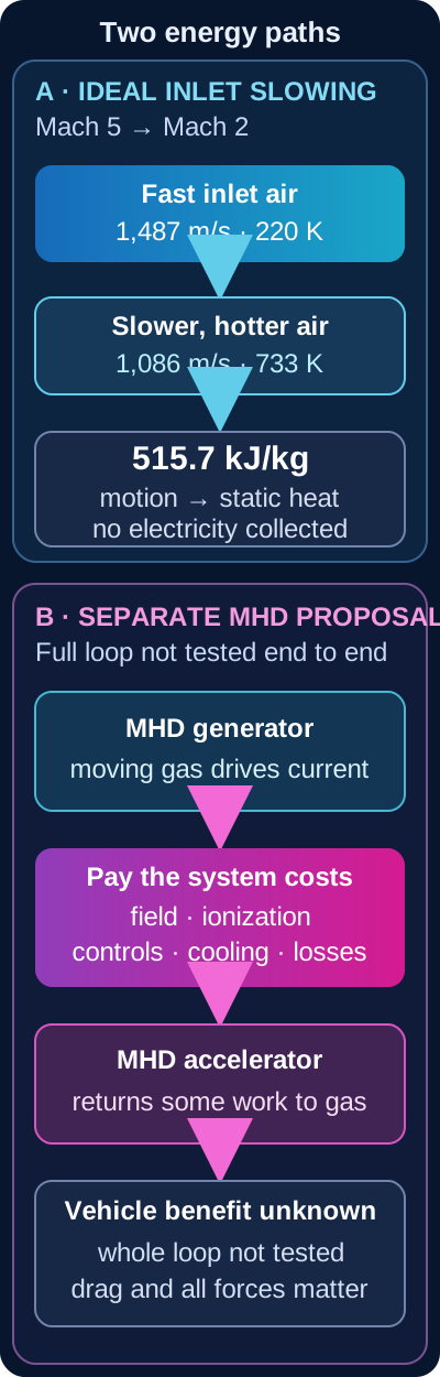
What this cannot show: no electrical output, usable-work fraction, coolant performance, fuel saving, combustion stability, net thrust or optimum shape is calculated. Heat moved into fuel through a wall is a different transfer from the inlet's conversion of flow kinetic energy into static enthalpy; the earlier regenerative-cooling diagram shows that separate path.
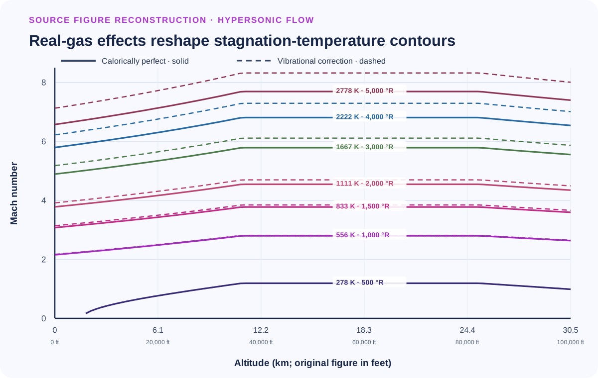
The curve is generated from the ideal-gas relation Tt/T = 1 + (γ − 1)M²/2 at fixed T = 220 K. It is an analytical reference, not measured flight data. The simulated outlet Mach number and pressure-recovery ratio are independent controls and are not guaranteed to describe one realizable inlet.
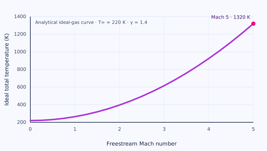
A DIFFERENT MHD EXPERIMENT / ONE DETONATION AT A TIME
Simple version: Researchers set off one carefully prepared gas pulse in a tube. The hot, electrically conducting gas passed through a small channel beside a magnet. Instruments measured current; researchers added up the electrical energy from that brief pulse. This helps test a generator component. It does not show an aircraft recovering energy in flight.
What was tested: NASA’s laboratory study used a single-cycle pulse-detonation device with an acetylene/oxygen mixture and a cesium-hydroxide seed dissolved in alcohol. The attached continuous-electrode Faraday channel produced measured current waveforms. The paper reports an effective gas conductivity of about 6 S/m for its diagnostic measurements. This is a distinct apparatus and experiment from the HVEPS scramjet tests described above.
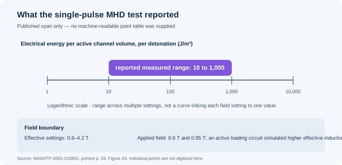
| Question | Evidence in the report | Boundary |
|---|---|---|
| Electrical energy | Measured range of about 10–1,000 J/m³ per detonation across effective-induction settings from 0.6 to 4.2 T | Energy per active channel volume for a pulse; the upper effective field was simulated by an active loading circuit, not supplied as the applied magnet field. |
| Applied field | 0.6 T and 0.95 T physical field settings; Figure 24 lists effective values through 4.2 T | Solid graph symbols mark conditions where applied B equals effective B. Do not describe every plotted field as a directly applied magnet field. |
| Thrust | The authors report negligible effect of MHD interaction on measured apparatus thrust because conductivity and enthalpy extraction were low. | It did not demonstrate a useful MHD thrust gain. The reported ~200 s apparatus specific impulse is not an MHD-caused improvement over the separately calculated ~120 s equivalent nozzleless-rocket comparison. |
| Scale-up | The authors calculate an illustrative 60 J per detonation and 6 kW at 100 cycles/s for a larger assumed channel. | Projection based on assumed channel dimensions, field, seeding and reduced electrode loss; it was not the laboratory output or a demonstrated continuous system. |
Why it is useful: the experiment shows how a short electrical waveform can be integrated into a per-pulse energy-density measure, and how load matching and near-electrode losses shape the result. It gives a concrete lesson for generator design and measurement methods. Its relevance to hypersonic flight is indirect: a single-pulse, laboratory detonation generator is not an air-breathing scramjet, and the study does not close a generator-to-accelerator loop or an aircraft energy/force balance.
Litchford, NASA/TP-2001-210801 (2001), NASA Technical Reports Server record · Full report PDF. Figure 24’s measured markers are plotted with theoretical curves in the source. This site redraws only the aggregate reported range because the report does not provide the individual values as a machine-readable table.
A SEPARATE HYPOTHESIS / FOLLOW THE ELECTRICAL BYPASS
This deliberately separate ledger shows the accounting structure of a proposed magnetohydrodynamic (MHD) bypass. It does not take energy from the 515.7 kJ/kg inlet example. Instead, you choose an assumed amount of stream energy that might be available to a generator, the fraction extracted, conversion efficiencies and auxiliary loads. These are teaching inputs, not measured MHD operating values.
For the strongest fully tabulated HVEPS case, the primary report separates 6.52 kW dissipated at the measured load bank from 14.38 kW estimated for the active channel after end-loss correction and 14.80 kW calculated as the matched-load maximum. The public AFRL 2-10-kW range does not specify enough detail to map it to one Table VI column. These component results do not establish vehicle net power or a complete bypass engine. Retained third-party indexed preprint copy; selected Table VI rows checked against the official NTIS/NTRL PDF · Official NTIS/NTRL report record and PDF.
Imagine trying to steer a stream of tiny moving particles with a magnet. The magnet can influence the flow more strongly when the gas carries electric current easily. How fast the air moves and how thin it is also matter. This old calculation explores those conditions; it does not show that an aircraft could fly there.
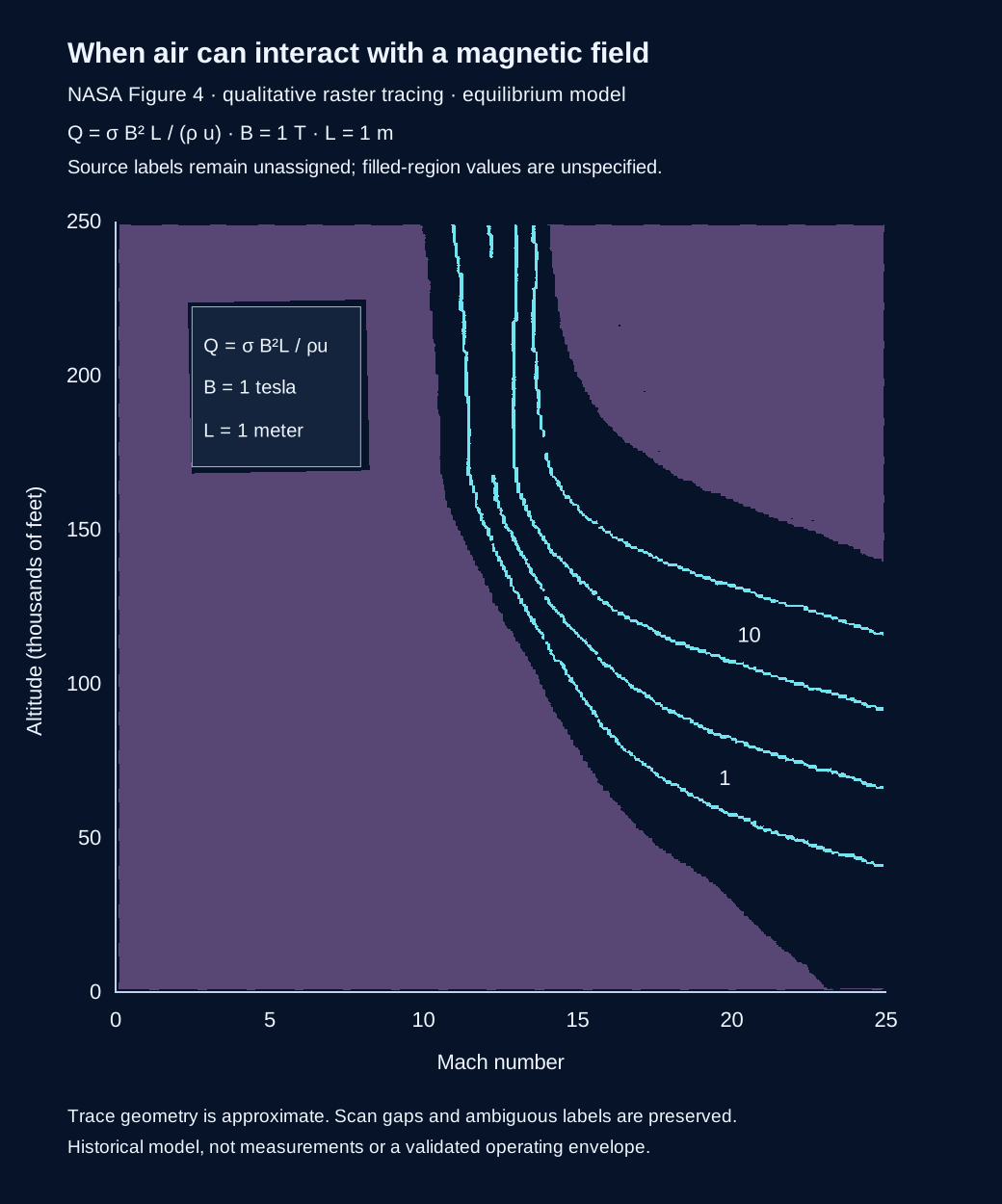
A map like this helps researchers ask where electromagnetic flow interaction deserves closer study. Reliable answers could inform energy conversion or flow-control research, but this figure alone demonstrates neither a useful device nor cleaner, cheaper or faster transport.
The source plots a dimensionless interaction parameter Q = sigma B squared L / (rho u), comparing an electromagnetic interaction scale with the flow's inertia. Its stated reference values are B = 1 tesla and L = 1 metre, with a 1976 Standard Atmosphere and equilibrium air behind a normal shock. Q is not electrical power or conversion efficiency. It cannot establish a net propulsion benefit without the rest of the flow, circuit, thermal and vehicle budgets.
The drawing follows a scanned figure rather than the original numerical arrays. It is not a recalculation of the modified chemical-equilibrium and transport solver, a CAD design, or an experimental operating envelope. No quantitative interpolation should be performed on unidentified contours.
In the formula, sigma is electrical conductivity, B is magnetic field strength, L is a characteristic length, rho is gas density and u is flow speed. None of the purple areas is labelled as a safe flight zone.
Drawing · SVG · Tracing method · JSON · Source pixel geometry · JSON, not physical data
The very simple version: It is not enough to know that electricity can move through a gas. We also need to understand which way it moves when a magnetic field is present. This graph describes one part of that behaviour in a calculation.
The Hall parameter β is dimensionless. Here it describes the relative importance of the Hall response in the source equations. It is different from conductivity, extracted power and efficiency. The source calculations concern equilibrium air behind a normal shock, at a fixed magnetic field of 1 tesla and two altitudes.
Scroll sideways on small screens or open the full-size figure.
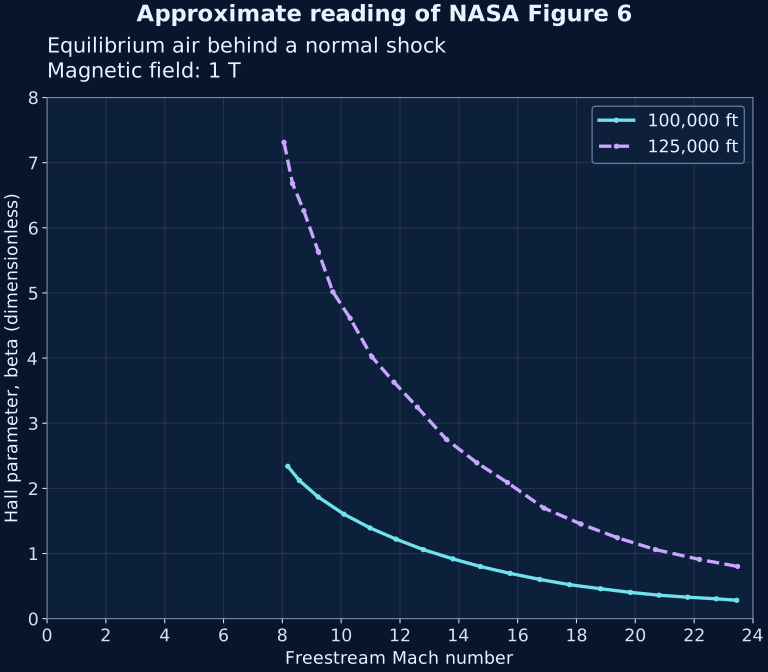
An unresolved source difference: at Mach 10 and 125,000 ft, the preceding report text says β is approximately 7, while the plotted curve reads approximately 4.8 here. We follow the graph and retain this disagreement. The original numerical values and the reason for the difference remain unverified; we do not correct the report or claim a new scientific finding.
Why this matters: assessing an electrical-energy concept needs the direction and distribution of current as well as its size. A conductivity estimate alone cannot establish the performance of an integrated system.
The pixel calibration accounts for the scan's slight skew. Each sample uses the centre of a visible dark run in the image. Project reading allowances are ±0.15 Mach and ±0.12 in β; these are graph-reading allowances, not statistical confidence intervals or uncertainty in NASA's model. Two coarse Mach-10 source checks agree within their broad visual ranges. This is not an independent equilibrium-air calculation.
The source's two altitude cases are 100,000 ft and 125,000 ft. The falling curves describe these particular calculations; they do not establish a universal relationship between speed and Hall response. No generated power, net thrust benefit or complete-engine feasibility is inferred.
Approximate points and source pixels · CSV · Calibration and limits · JSON · Replot from CSV · Python. Place the CSV next to the script; matplotlib is required.
| Altitude (ft) | Mach | β |
|---|---|---|
| 125000 | 8.06 | 7.31 |
| 125000 | 8.35 | 6.68 |
| 125000 | 8.73 | 6.26 |
| 125000 | 9.22 | 5.63 |
| 125000 | 9.72 | 5.02 |
| 125000 | 10.31 | 4.61 |
| 125000 | 11.05 | 4.02 |
| 125000 | 11.80 | 3.63 |
| 125000 | 12.59 | 3.25 |
| 125000 | 13.58 | 2.75 |
| 125000 | 14.62 | 2.39 |
| 125000 | 15.66 | 2.09 |
| 125000 | 16.89 | 1.70 |
| 125000 | 18.14 | 1.45 |
| 125000 | 19.39 | 1.24 |
| 125000 | 20.68 | 1.06 |
| 125000 | 22.18 | 0.91 |
| 125000 | 23.48 | 0.80 |
| 100000 | 8.19 | 2.34 |
| 100000 | 8.58 | 2.12 |
| 100000 | 9.22 | 1.87 |
| 100000 | 10.10 | 1.60 |
| 100000 | 10.98 | 1.39 |
| 100000 | 11.86 | 1.22 |
| 100000 | 12.79 | 1.06 |
| 100000 | 13.80 | 0.92 |
| 100000 | 14.73 | 0.80 |
| 100000 | 15.74 | 0.70 |
| 100000 | 16.75 | 0.60 |
| 100000 | 17.76 | 0.52 |
| 100000 | 18.82 | 0.46 |
| 100000 | 19.83 | 0.40 |
| 100000 | 20.81 | 0.36 |
| 100000 | 21.78 | 0.33 |
| 100000 | 22.76 | 0.30 |
| 100000 | 23.45 | 0.28 |
The very simple version: Electricity needs moving charged particles. How easily it travels through a gas depends on what is in the gas and its state. These pictures compare two calculated gas compositions. They do not compare two working engines.
The upper panel is equilibrium air; the lower includes a cesium seed fraction specified by the historical study. Each compares two altitudes. The source attributes the dips to molecular dissociation. These are published calculations for gas behind a normal shock, not flight measurements or a recommendation for a practical mixture.
On small screens, scroll sideways inside the figure or open it full-size.
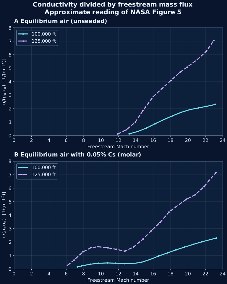
Why this matters: checking gas conductivity helps assess an energy-conversion concept before committing to complex hardware. A favourable trend still needs a complete accounting of energy, electrical demands and equipment mass.
The vertical axis is σ/(ρ∞u∞), conductivity divided by freestream mass flux, with units 1/(m·T²). T here denotes tesla. It is not power, conversion efficiency or the dimensionless interaction parameter Q. Converting it to Q requires B²L and a compatible local-versus-freestream mass-flux convention.
The source compares 100,000 ft and 125,000 ft, and a lower-panel seed fraction of 0.05% cesium by mole. It describes a modified NASA SP-273 equilibrium calculation with Frost transport methodology. The original numerical arrays and exact solver configuration are not reproduced here.
Each panel has its own linear pixel calibration accounting for scan skew. Selected samples were checked against dark trace pixels, and eight coarse source readings provided a comparison. Two comparisons were reread after an initial disagreement; this was not a wholly blind validation. Project graph-reading allowances are ±0.3 Mach and ±0.1 in the ordinate units, not statistical confidence intervals or uncertainty in the physical model. The data file retains the pixel coordinates.
Approximate readings · CSV · Calibration and limits · JSON · Replot from the CSV · Python. Put the CSV beside the script; matplotlib is required.
| Panel | Altitude (ft) | Mach | Normalized conductivity |
|---|---|---|---|
| unseeded | 100000 | 13.232 | 0.124 |
| unseeded | 100000 | 14.222 | 0.301 |
| unseeded | 100000 | 15.218 | 0.556 |
| unseeded | 100000 | 16.217 | 0.876 |
| unseeded | 100000 | 17.215 | 1.183 |
| unseeded | 100000 | 18.212 | 1.465 |
| unseeded | 100000 | 19.207 | 1.72 |
| unseeded | 100000 | 20.199 | 1.923 |
| unseeded | 100000 | 21.187 | 2.048 |
| unseeded | 100000 | 22.174 | 2.173 |
| unseeded | 100000 | 23.162 | 2.311 |
| unseeded | 125000 | 11.926 | 0.118 |
| unseeded | 125000 | 12.925 | 0.438 |
| unseeded | 125000 | 13.938 | 0.993 |
| unseeded | 125000 | 14.807 | 1.848 |
| unseeded | 125000 | 16.014 | 2.897 |
| unseeded | 125000 | 17.031 | 3.504 |
| unseeded | 125000 | 18.047 | 4.097 |
| unseeded | 125000 | 19.063 | 4.691 |
| unseeded | 125000 | 19.903 | 5.078 |
| unseeded | 125000 | 21.08 | 5.645 |
| unseeded | 125000 | 22.097 | 6.251 |
| unseeded | 125000 | 22.963 | 7.054 |
| seeded | 100000 | 7.275 | 0.156 |
| seeded | 100000 | 7.769 | 0.231 |
| seeded | 100000 | 8.757 | 0.356 |
| seeded | 100000 | 9.741 | 0.429 |
| seeded | 100000 | 10.721 | 0.45 |
| seeded | 100000 | 11.7 | 0.432 |
| seeded | 100000 | 12.678 | 0.4 |
| seeded | 100000 | 13.658 | 0.408 |
| seeded | 100000 | 14.642 | 0.494 |
| seeded | 100000 | 15.635 | 0.71 |
| seeded | 100000 | 16.631 | 0.965 |
| seeded | 100000 | 17.624 | 1.194 |
| seeded | 100000 | 18.618 | 1.423 |
| seeded | 100000 | 19.61 | 1.626 |
| seeded | 100000 | 20.602 | 1.83 |
| seeded | 100000 | 21.593 | 2.02 |
| seeded | 100000 | 23.243 | 2.297 |
| seeded | 125000 | 6.139 | 0.266 |
| seeded | 125000 | 6.898 | 0.666 |
| seeded | 125000 | 7.915 | 1.273 |
| seeded | 125000 | 8.831 | 1.581 |
| seeded | 125000 | 9.652 | 1.654 |
| seeded | 125000 | 10.79 | 1.57 |
| seeded | 125000 | 11.763 | 1.461 |
| seeded | 125000 | 12.734 | 1.325 |
| seeded | 125000 | 13.733 | 1.632 |
| seeded | 125000 | 14.83 | 2.226 |
| seeded | 125000 | 15.765 | 2.833 |
| seeded | 125000 | 16.783 | 3.453 |
| seeded | 125000 | 17.81 | 4.229 |
| seeded | 125000 | 18.652 | 4.641 |
| seeded | 125000 | 19.827 | 5.182 |
| seeded | 125000 | 20.827 | 5.516 |
| seeded | 125000 | 21.843 | 6.109 |
| seeded | 125000 | 22.359 | 6.524 |
| seeded | 125000 | 23.214 | 7.157 |
This figure establishes neither a demonstrated complete propulsion loop nor a net energy gain. The gas model, electrical conversion and integrated vehicle performance are different questions.
The very simple version: Slowing very fast air can make it hotter. This model asks whether taking some energy out first could let the air enter the burner more slowly without becoming too hot. Passing that one check does not mean the whole engine will work.
Ramjet combustion uses subsonic flow; scramjet combustion uses supersonic flow. The curve below marks a burner-entry Mach number of one in a simplified temperature constraint. It is a conditional reconstruction of Eq. (71), in the context of NASA Figure 3, rather than a digitization of the original curve or a demonstrated flight envelope. Its short dashed tail marks calculated values beyond the end of the source curve, which is only visually readable to about extraction ratio 0.78.
Scroll sideways on small screens or open the full-size figure.
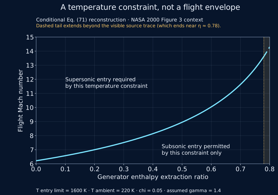
| Extraction ratio | Boundary flight Mach |
|---|---|
| 0 | 6.22 |
| 0.4 | 8.14 |
| 0.8 | 14.30 |
At the boundary, Mₐ = √{[2/(γ − 1)] × [((γ + 1)/2)(T₃,lim/Tₐ)(1 − χη)/(1 − η) − 1]}, where η is the generator enthalpy-extraction ratio. The code evaluates η from 0 to 0.8; it does not approach the singular limit at one.
Four separate approximate readings of the source graph are consistent with this reconstruction within project-selected visual allowances. That comparison does not validate the physical model or establish exact reproduction. The visible source curve ends near extraction ratio 0.78 by approximate raster reading. The styled graph changes to a dashed line beyond that point to mark the calculated extension to 0.8; this is not an exact source endpoint measurement.
Why this matters: a promising temperature trend must still be checked against electrical demands, gas properties, pressure losses and the rest of the engine. The lower plotted region only passes this temperature constraint; it does not prove a complete flow solution, stable combustion, net thrust benefit or practical MHD extraction. No full-engine design or flight prediction follows from this chart.
Calculated values · CSV · Graph image · PNG · Assumptions and checks · JSON · Reproduce the calculation and figure · Python
The very simple version: Imagine taking some energy from a fast stream, carrying it along a wire, then giving some of it back farther downstream. The two pictures follow the same proposed cycle: one follows the components, the other follows the gas state. Every transfer still has losses.
The upper panel preserves the source station labels. The lower panel is an enthalpy–entropy sketch: height represents enthalpy and horizontal position entropy. Curved pressure guides and the dashed temperature-limit line are qualitative. They are not measured trajectories or numerical performance data.
On a small screen, scroll sideways inside the figure or open the full-size redraw. Compare it with the original NASA Figure 1 crop (PNG).
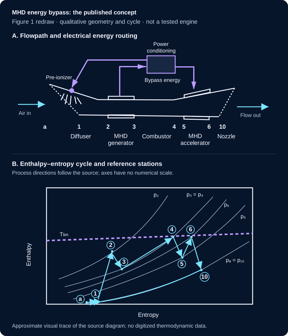
What it can help us understand: energy moves between components, so a gain in one part cannot be judged without the losses and demands elsewhere. This drawing explains a simplified thermodynamic concept. It does not establish that a complete bypass engine has been built, that the assumed states are achievable, or that net vehicle performance improves.

PUBLISHED CONCEPT · 1995 · MODEL, NOT DEMONSTRATED ENGINE
In everyday words: a rocket engine could share some energy from its hot exhaust with a second stream of air passing around it. The second stream might add momentum to the combined exhaust. The energy still comes from the rocket's propellant; it is not free energy or a self-powering loop.
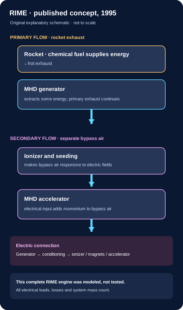
| Evidence | What the source reports | What it does not establish |
|---|---|---|
| Conventional rocket ejector test · 1995 | The paper summarizes ground tests of thermodynamic ejectors. One reported configuration had about 54% thrust augmentation at a secondary-to-primary mass ratio near 3.7 in a thermodynamic RENE configuration simulated for 40,000 ft and Mach 2, with L/D = 2 and feather-cut mixing aids. | This was not an MHD generator-and-accelerator test and does not measure RIME performance. |
| RIME model and vehicle sizing · 1995 | The authors modeled an MHD ejector and used assumed performance values in a first-order vehicle study. Their example assigned very large masses to the generator and accelerator/ionizer and described a hypothetical generator/power scale around 1 GW for its example. | No integrated RIME engine test or flight result. These are study assumptions and calculations, not measured performance or a validated design. |
| NASA program review · 1997 | A later NASA review describes performance-code development connected with a RIME study. | Code development is not a component experiment or an integrated propulsion demonstration. |
| PDRIME follow-on concept · 2008 | A later pulse-detonation variant reports numerical modeling of a related concept. | The located record is not evidence of a tested or flown integrated PDRIME engine. |
The 1995 paper's architecture contains a rocket engine, MHD generator, ionizer and MHD accelerator. Its electrical path links generator output to downstream loads; the accelerated secondary flow is distinct from the primary rocket exhaust until mixing. A vehicle benefit cannot be inferred from generator output alone: the control volume must include primary-flow energy and momentum removed by the generator, every electrical load and conversion loss, secondary-air momentum, mixing, pressure thrust and installed mass.
The paper also notes the demanding electrical-power and mass implications, and recommends laboratory testing and further computational/system studies. This section therefore records a published hypothesis and its proposed evaluation path, not a validated technology. The source report warns that its own vehicle study omitted important factors including sea-level pressure and landing capability.
Sources: Cole, Campbell & Robertson, Rocket-Induced Magnetohydrodynamic Ejector—A Single-Stage-to-Orbit Advanced Propulsion Concept, NASA-TM-111435 / AIAA 95-4079 (1995), NASA NTRS record · NASA-hosted report PDF; NASA CR-97-206242/PT1 (1997), NASA NTRS record. The 2008 PDRIME item is listed only as a related modeling study: author-uploaded paper record · UCLA publication listing.
Copyright/reuse note: the 1995 report carries a notice reserving non-US rights and directs republication inquiries to AIAA. Its source artwork is not reproduced here. The diagram above is an original explanatory schematic; broader rights in close recreation of source figures were not assessed.

These are related but different pieces of evidence. A component test is not an integrated engine test, and a cycle model is not a flight result.
In everyday words: the JAXA computer study tried slowing the air with a magnetic force to change the shock in the inlet. One pressure loss became smaller, but the generator still took momentum from the air, so the total pressure went down. The team calculated the inlet and the pushing nozzle separately; they did not show the two parts working together.
| Evidence | What was studied or measured | What it tells us | What it does not establish |
|---|---|---|---|
| NASA cycle analysis, 2000 | Simplified thermodynamic model of an MHD generator and downstream accelerator, using idealized gas assumptions. | A bypass loop can be written as a cycle model; the model examined possible operating envelopes. | The paper notes that non-isentropic MHD losses hamper overall performance. It is not a built or flown engine. NASA Technical Paper 2000-210387. |
| Riggins cycle simulation, 2002 | Full-cycle simulations at high Mach numbers, as described by the NASA record abstract. | The abstract reports that the simulated system underperformed a conventional scramjet in the studied cases, with total-pressure loss and irreversibility identified as important concerns. | The full report and numerical data were not available for this review; no graph or exact values are reproduced. NASA record 20020073109. |
| Riggins peer-reviewed journal analysis, 2004 | Thermally balanced MHD-bypass and conventional-scramjet simulations, including inlet shocks, chemistry, wall cooling, fuel injection/mixing and friction. | The abstract reports lower modeled MHD-bypass performance across Mach 8–12.2, attributing it to added MHD irreversibility/cooling and inverse-cycle total-pressure reduction. | The institutional record identifies a peer-reviewed journal article, but exposes citation/abstract only; full paper and numerical curves remain unavailable for this review. It is related to, but must not be merged with, the simplified NASA 2000 Figure 2. Official English journal record · Missouri S&T record. |
| Kaminaga et al., MHD-bypass scramjet model, 2005 | Steady quasi-one-dimensional Mach-8 numerical comparison at a nominal 30 km atmosphere. The paper accounts for combustor pressure contribution, wall friction and generator Lorentz-force momentum change; it routes all modeled generator electrical output to the downstream accelerator. | Simple version: slowing the air can help the burner and change the pressure forces, but the generator pushes back on the flow. In this model, those effects nearly cancel: the authors report about a 3% normalized net-thrust change. The strongest modeled setting chokes after fuel is added. Technical result: Fig. 12's approximate visual readings span 0.977–1.036 of baseline; these are not raw table values or an uncertainty interval. | This is a calculation, not a test or flight result. It assumes unit inlet capture, chemical equilibrium, no mixing delay, adiabatic walls and 80% electrical and accelerator efficiencies; oblique inlet shocks are not explicitly modeled. Approximate graph readings are not a raw data table or an uncertainty analysis. Journal article · Full paper, Fig. 12 (PDF p. 7; printed p. 560). |
| Maehara & Suzuki, JAXA numerical study, 2009 | Two-dimensional Euler/MHD intake calculations at a Mach-5 design point, including a Mach-6 off-design case at a nominal 30 km altitude. The model assumes 10 S/m electrical conductivity through seeding and applies a 0.1 T magnetic field in its main 2-D case. | The modeled Lorentz force changes the shock and can reduce pressure loss across the shock. Yet total pressure still decreases overall because the generator brakes the flow; the reported total-temperature reduction is small and does not remove the wall-heating issue. A separate nozzle calculation reports acceleration. | The inlet generator and nozzle accelerator were analyzed separately, with different modeled conditions; they were not a simultaneously coupled cycle, measured system or flight test. Conductivity is an imposed assumption. The paper says full inlet/combustor/nozzle coupling is needed. Its nozzle table prints an electric-field unit as “500 [V]”; the source's unit/quantity is ambiguous, so it is left unresolved. JAXA repository record · JAXA-hosted paper PDF (6 pages). |
| HVEPS hot-flow ground demonstration | A scramjet combustor test rig fed an inline MHD generator downstream of the combustor at Mach-8-simulating conditions. | The full AFRL preprint reports seven brief powered tests. For Test 3 it reports 6.52 kW dissipated at the load bank; post-test analysis gives 14.38 kW active-channel output after excluding end losses and a calculated 14.80-kW maximum at matched load. General Atomics separately reports a preliminary 15-kW peak over the active section. AFRL's public 2-10-kW range does not specify enough detail to map it to a particular Table VI column. Retained third-party indexed preprint copy; selected Table VI rows checked against the official NTIS/NTRL PDF | AFRL program summary | AIAA paper DOI | General Atomics release. | Component ground-test output only; no complete accelerator loop, aircraft power-bus closure, or flight thrust benefit. |
| MAPX accelerator facility design and status | A separately powered arc-heated hypersonic-flow research facility and MHD accelerator. NASA’s 2003 design point lists 1.3 MW applied electrical power, 61 kW predicted MHD push work and about 150% calculated velocity augmentation. | These are facility design/model values, not a measured accelerator output or thrust gain. The 2003 report describes hardware integration and planned shakedown; the 2008 NASA status abstract reports preliminary tests and progress toward full-up assembly, without a quantitative completed-run result. | MAPX was a different externally powered accelerator program. It does not validate the HVEPS combustor-exhaust generator, an aircraft generator-to-accelerator bypass loop, or a self-excited net-positive flight system. NASA/TP-2003-212285 design report · NASA 2008 MAPX status record. |
| Ling et al., scramjet MHD generator-channel simulation, 2024 | A Fluent-based numerical model for one scramjet MHD power-generation channel, with magnetic-field cases from 1 to 4 T. | The publisher abstract reports generation efficiency of 22.5–21.5% and enthalpy extraction of 0.026–0.34% across those cases, with opposite trends as field rises. The abstract names two distinct quantities but does not define their denominators. Their exact relationship remains unverified here; neither percentage establishes whole-engine net efficiency. | Abstract-level transcription only; definitions, benchmark, full assumptions and independent reproduction remain to be checked in the full article. Channel simulation, not measured generator output, closed energy bypass, or whole-engine net efficiency. Official English journal record · Publisher abstract. |
| Liu, Wu & Meng, post-combustor MHD generator model, 2025 | A baseline scramjet performance model checked against Mach 7 / 29 km test-point data, then coupled to an analytical post-combustor MHD generator model. | At 0.5% enthalpy extraction, a 2.5 T field and load factor 0.4, the paper reports a 3.58% specific-impulse penalty for the modelled MHD stage. | The check against flight-point engine data concerns the baseline model; MHD generation itself is modeled, not experimentally integrated. The configuration is post-combustor power extraction, not proof of an inlet-generator/accelerator loop. Full paper must be independently reproduced before using the result as validation. Official English journal record · Publisher record. |
| Benyo, NASA NPSS MHD-turbojet cycle, 2011 | A coupled thermodynamic cycle model connects a pre-ionizer and MHD generator upstream of a supersonic turbojet with a second pre-ionizer and MHD accelerator downstream. For its Mach 3.25–7 cases it uses a 3 m generator, 2.5 T field and 2–5.5 S/m conductivity. | The model reports 45–90 MW extracted electrically and positive specific net thrust from 740 N·s/kg at Mach 3.25 to 70 N·s/kg at Mach 7. It allocates 90% of generated power to the accelerator and 5% to each pre-ionizer. These are model outputs, not engine measurements. | This is a genuine integrated cycle simulation for a turbojet, not a scramjet or tested propulsion system. The generator is modeled at an assumed 90% isentropic efficiency; conductivity is prescribed. The report leaves vehicle sizing and cost-benefit analysis for future work, so magnetic-system mass, drag, cooling and hardware-level feasibility are not closed. NASA NTRS record · Full NASA/TM-2011-217136, printed pp. 1–13 (PDF pp. 5–17) · Source-value graph. |
| Schneider, annular Hall-MHD turbojet cycle, 2011 | A preliminary 1-D axisymmetric model iterates an MHD generator and accelerator with a Mach-7, 30 km turbojet. The generator calculates 1.6 MJ/kg extraction at 5 T, 5 S/m and 3 m; after ionizer allocation, about 1.4 MJ/kg is passed to the 3 m accelerator calculated at 5 T and 1 S/m. | The preliminary cycle estimates 185 N·s/kg positive thrust per unit mass flow. It calculates 84% generator and 81% accelerator isentropic efficiencies and a very large generator total-pressure drop, from 2,350 to 18 kPa. | These are calculations, not measured thrust or power. The estimated ionization fraction for 1–5 S/m is about 2–3 orders above the cited discharge estimate; the report calls for improved 2-D/3-D modeling and designed generator/accelerator experiments. Do not treat its high component efficiencies as achieved hardware performance. NASA NTRS record · Full NASA/TM-2011-217210, pp. 7–15. |
What the models disagree on: a NASA NPSS turbojet model predicts positive net thrust for its chosen MHD assumptions; a fully thermally balanced MHD scramjet analysis predicts lower performance than a conventional scramjet in its Mach 8–12.2 cases; a separate 2005 scramjet model reports no significant net-thrust difference. These are different modeled engines and assumptions, not competing flight tests. No one result settles whether an atmospheric MHD energy-bypass vehicle is useful.


| Generator interaction parameter, sgen | Normalized net thrust (baseline = 1) | Reading status |
|---|---|---|
| 0.00 | 1.000 | Approximate graph reading |
| −0.05 | 0.981 | Approximate graph reading |
| −0.10 | 0.977 | Approximate graph reading |
| −0.15 | 0.990 | Approximate graph reading |
| −0.20 | 1.022 | Approximate graph reading |
| −0.25 | 1.036 | Approximate graph reading |
| −0.30 | 1.026 | Approximate graph reading |
| −0.35 | 1.002 | Approximate graph reading |
| −0.40 | No normalized value plotted | Fuel injection choked the flow; authors report no useful thrust. |
Visual readout tolerance on numeric points: approximately ±0.002, not model/experimental uncertainty. Download the CSV to preserve the same values and status.
Simple version: The generator slows the air and takes energy out. That makes one part of the engine push harder and can lower wall drag, but the same slowing force pushes back against the air. In this published calculation, those gains and losses nearly cancel. One case also becomes blocked when the model adds fuel. The graph is from a computer calculation, not an airplane test.
To find out whether the loop could help a vehicle, a coupled study would need the same operating point and a consistent account of inlet state, mass flow, electrical conductivity, generator pressure loss, magnet mass and power, cooling, combustion, accelerator efficiency, nozzle performance, installation weight, drag and mission fuel. The current ledger is a transparent arithmetic exercise; it does not contain those linked data, so it cannot calculate net thrust or a vehicle benefit.
The hypothetical flow-energy scale is an independent teaching input per kilogram. It is not thermodynamic availability (exergy), is not derived from the inlet state, and is not the inlet's 515.7 kJ/kg energy conversion. It is not evidence that a real generator can access the selected amount. For this bookkeeping boundary, generator and accelerator conversion losses are treated as unavailable to the modeled gas stream (as if rejected outside it); any loss heat returned to the gas is not modeled.
What “self-excited” means: in some MHD generator architectures, generator output helps establish or sustain the electromagnet field (for example through a capacitor or field circuit). That power is part of the energy budget, and startup can depend on residual/seed field and circuit conditions. Electrodes do not create free excitation. Energy stored in the field is measured in joules; ongoing power is measured in watts. The slider below represents an assumed average operating demand, not a calculation of start-up energy or a universal cost for every type of magnet. That operating demand is assigned alongside other auxiliary demand before power is sent to the accelerator. Background: magnetic-field energy and power. If generated power cannot meet both demands, this simplified model reports their combined shortfall but does not allocate it between them. It does not model magnetic-field startup or dynamics. Published examples are machine-specific: a NASA liquid-metal MHD spacecraft power-system design used shunt-capacitor excitation; a separate NASA pulse-detonation/MHD study reports small-scale tests; and a liquid-metal generator study found startup depended strongly on residual magnetic field. None demonstrates a hypersonic flight generator-to-accelerator loop. See the NASA power-system design, NASA pulse-detonation/MHD study, and liquid-metal startup study.
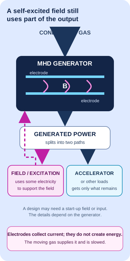
A SEPARATE NASA CONCEPT · ATMOSPHERIC ENTRY CONTROL
Simple version: A very fast spacecraft can heat and ionize the air around it. NASA researchers modelled placing electrodes in that conducting flow to collect an electric current, then using it to power a magnet. The magnet and current could push on the surrounding flow to help steer the spacecraft during atmospheric entry.
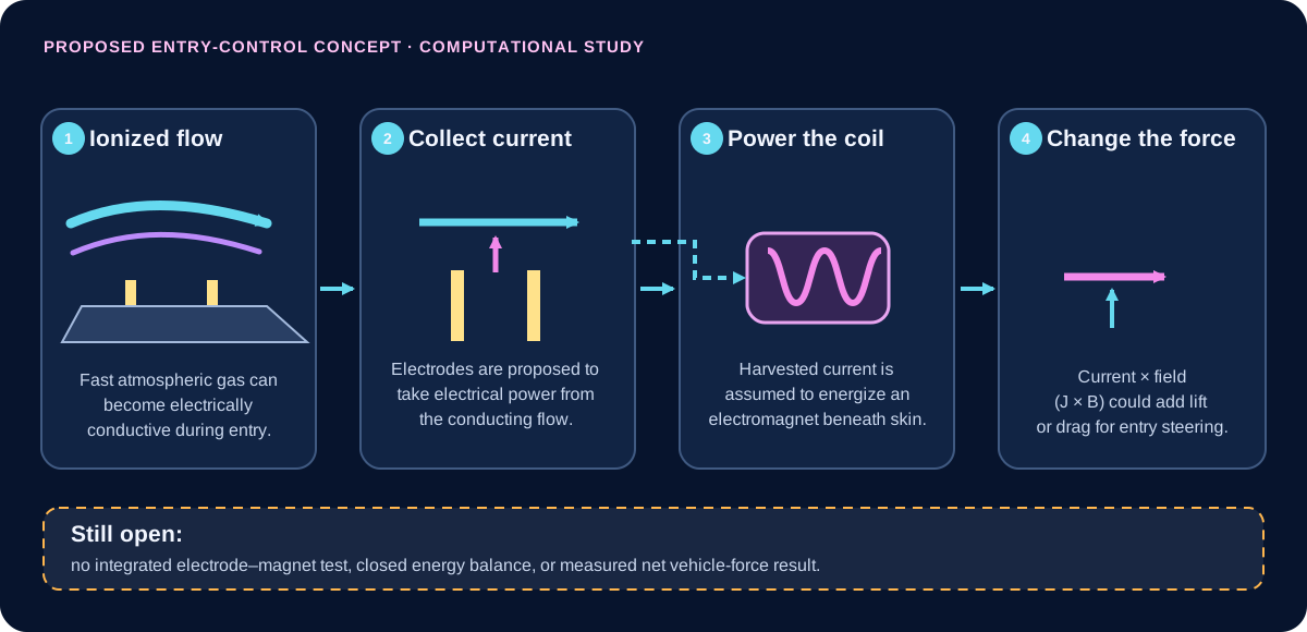
What the study actually did: its computational workflow first calculated an atmospheric-entry flow with NASA’s LAURA code, then used CFDWARP to estimate current paths and Lorentz forces for an MHD patch. The second calculation treated the temperature, velocity and density from the first as fixed inputs; the paper says this case had “no coupling.” It assumes harvested electrical power can run the electromagnet rather than demonstrating a working electrode-to-coil assembly in a test.
The paper’s Mars example illustrates why corrections matter: after accounting for Hall, ion-slip and three-dimensional effects, the computed forces were on the order of 20 kN for the 1 T case, compared with 709 kN conventional aerodynamic drag in that model. The authors list flight-mechanics and thermal-load work still needed before flight demonstration. NASA’s technology-transfer page separately summarizes an in-silico Neptune-entry estimate of up to 200 kN from a 1 m² patch; it is not a measured force.
How this relates to the 515.7 kJ/kg example: the earlier number is an ideal calculation of inlet-flow kinetic energy converted into static enthalpy for a perfect-gas Mach 5 to Mach 2 example. It is not measured electrical output. The NASA entry-control concept is a different flow, mission and purpose; it does not show that this inlet-energy amount can be collected and returned to a hypersonic engine or that thrust increases.
To validate the proposed feedback, a test would need synchronized plasma/flow measurements, electrode output, coil startup and steady power, magnetic-field strength, all electrical and thermal losses, the change in flow and vehicle force, and a complete uncertainty-bounded energy balance.
Primary sources: NASA Langley et al., “New Magnetohydrodynamic (MHD) Lift Concept for More Efficient Missions to Mars and Neptune” (methods PDF pp. 6–7; Mars result p. 11; future work pp. 12–13) · NASA Tech Transfer, LAR-TOPS-363 (states the 200 kN value is from in-silico entry evaluation).
With the reference settings, 5.83% extraction just covers the assumed 35 kW of loads; zero power reaches the accelerator at that point.
The ledger estimates this threshold as fcover = (Paux + Pfield) / (ṁ q ηg). It is only a threshold inside this hypothetical stream-energy ledger. The chosen q is not a measured reservoir or guaranteed extractable energy.
In ordinary decimal units, the assumed loads total 20 + 15 = 35 kW, and the hypothetical generator output at 100% extraction would be 10 kg/s × 100 kJ/kg × 60% = 600 kW. So the exact ratio is 35/600 = 7/120 = 5.833…%.
Writing that same ratio in base 12 gives 7/A012, or 5.A12%. This changes the notation, not the underlying measurements, assumptions, precision or physics; it does not improve the estimate.
Boundary of this number: At the reference settings, −149 kW is the change in this model’s stream-energy account only. It is not whole-engine net power, net thrust or a measured propulsion gain. The model does not include the pressure, momentum, drag, heat-rejection, structural or vehicle-level effects needed to calculate those outcomes.
515.7 kJ/kg follows from one stated perfect-gas example. It is a calculated state change, not collected electricity.
Published analyses explore generator and accelerator paths. Results depend on assumptions, pressure losses and conversion costs.
A separate hot-flow ground test produced electrical output from an MHD generator component. It did not test a complete engine.
Laboratory accelerator research is a distinct evidence class; it is not an integrated bypass flight test.
No matched flight result here demonstrates net thrust, fuel or mission improvement from the complete loop.
A useful next test, not yet reported: compare a bypass and a baseline configuration at one matched operating point. Measure mass flow, inlet and exhaust total pressure, net thrust, generator output, field and auxiliary power, fuel flow, cooling and uncertainty.
These evidence classes are not steps that certify the next one. Open the study comparison and source links.
At the selected assumptions, this ledger removes power from the stream, deducts conversion and auxiliary costs, and returns only a fraction downstream.
Premoved = ṁ · qavailable · fextract
Pelectric = ηgenerator · Premoved
Ploads served = min(Pelectric, Paux + Pfield)
Paccelerator input = Pelectric − Ploads served
Preturned = ηaccelerator · Paccelerator input
Premoved − Preturned = generator loss + loads served + accelerator loss
Simple version: If all the energy missing from the stream came from its forward motion, the air would slow down. This small comparison shows the size of that possible change. It cannot tell us the real force on an MHD engine or aircraft.
For an assumed uniform flow with no added mass, divide the ledger's net stream-energy debit by its mass flow. Then assign that entire amount to bulk kinetic energy: Δe [J/kg] = 1,000 × Pdebit [kW] / ṁ [kg/s]; vout,eq = √(vin2 − 2Δe). This is a conditional energy-to-speed translation; pressure, heat and enthalpy changes are not solved.
Conditional illustration only: this assigns the entire modeled stream-energy debit to bulk kinetic energy in a uniform one-dimensional stream. It is not the MHD device's predicted force, drag, thrust or aircraft performance.
Reference example: with the ledger's default 149 kW debit and 10 kg/s flow, the debit is 14.9 kJ/kg. At an independently chosen 1,500 m/s, assigning all of it to kinetic energy gives an equivalent 1,490.03 m/s outlet and a −99.7 N plug-flow momentum-flux change. These are a teaching scenario, not measured or paired vehicle data. This is not the separate Mach-5-to-2 inlet result.
What a real vehicle balance still needs: captured and spilled air mass; inlet, generator, combustor and nozzle pressure/velocity/enthalpy states; forces on all internal and external surfaces; heat returned to the stream; fuel flow; installed hardware mass; and vehicle drag at the same flight condition. Without these matched measurements, the Site must not label the equivalent number as thrust or propulsion gain. The HVEPS 6.52 kW load-bank reading is a separate component result; without a matched channel mass flow and inlet/outlet state, it cannot be converted into this stream-speed comparison.
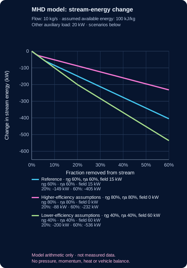
| Teaching scenario | Generator efficiency | Accelerator efficiency | Field debit | Change at 20% extraction | Change at 60% extraction |
|---|---|---|---|---|---|
| Reference | 60% | 60% | 15 kW | −149 kW | −405 kW |
| Higher selected efficiencies; no field debit | 80% | 80% | 0 kW | −88 kW | −232 kW |
| Lower selected efficiencies; 60 kW field debit | 40% | 40% | 60 kW | −200 kW | −536 kW |
Here “net stream-energy change” means only removed flow energy plus modeled accelerator work returned to the flow. It is not engine net power. The original 360-row file varies four controls at once; this chart instead isolates extraction fraction and holds each scenario's other inputs fixed.
This arithmetic does not model ionization chemistry, electrical conductivity, magnet mass, field power, heat rejection, shock structure, total-pressure loss, combustor matching, nozzle expansion or aircraft drag. It therefore calculates no thrust, net efficiency or vehicle benefit. A positive electrical output is not a positive whole-engine gain.
This uses the same illustrative ledger settings above: 10 kg/s flow (A₁₂), 100 kJ/kg assumed available energy (84₁₂), extraction fraction 1/5, generator and accelerator efficiencies 3/5, 20 kW auxiliary load (18₁₂), and 15 kW field demand (13₁₂). A and B stand for ten and eleven. The table recomputes the same exact integer-kilowatt results using the same rational fractions.
| Quantity | Decimal arithmetic | Same result in base 12 |
|---|---|---|
| Power removed from the stream | 10 × 100 × 1/5 = 200 kW | A × 84 × 1/5 = 148₁₂ kW |
| Generator electrical output | 200 × 3/5 = 120 kW | 148 × 3/5 = A0₁₂ kW |
| Auxiliary and field demand served | 20 + 15 = 35 kW | 18 + 13 = 2B₁₂ kW |
| Power sent to accelerator | 120 − 35 = 85 kW | A0 − 2B = 71₁₂ kW |
| Accelerator work returned to gas | 85 × 3/5 = 51 kW | 71 × 3/5 = 43₁₂ kW |
| Generator conversion loss | 200 − 120 = 80 kW | 148 − A0 = 68₁₂ kW |
| Accelerator conversion loss | 85 − 51 = 34 kW | 71 − 43 = 2A₁₂ kW |
| Stream-energy debit | 200 − 51 = 149 kW | 148 − 43 = 105₁₂ kW |
| Account closure | 80 + 35 + 34 = 149 kW | 68 + 2B + 2A = 105₁₂ kW |
Both notations close the same ledger exactly. This is a cross-check of arithmetic and place-value conversion only: it does not validate the chosen efficiencies, describe self-excitation dynamics, or predict a real MHD generator, thrust or aircraft benefit. Base 12 does not improve physical precision; SI source values remain in decimal.
Two hundred seventy deterministic combinations vary the extraction fraction, generator efficiency, accelerator efficiency and assumed field-excitation demand while holding other inputs fixed. The reference case removes 200 kW from the chosen stream, produces 120 kW at the generator terminals, assigns 20 kW to other auxiliaries and 15 kW to field excitation, leaving 85 kW at the accelerator and returning 51 kW as accelerator work. Thus the stream account falls by 149 kW; pressure and momentum consequences are not calculated. That 149 kW is not whole-engine net power or a measured propulsion gain. The ledger tracks an assumed stream-and-electric-energy boundary only; it omits the pressure, momentum, drag, thermal, structural and vehicle-level consequences needed to judge net thrust, range or fuel use. The example is arithmetic for stated assumptions, not a validated hypersonic engine.
TRY A BOUNDED MODEL / ONE IDEAL STREAM
Imagine removing a selected fraction of a stream's kinetic power, with its mass flow held constant. Both speeds and kinetic powers are measured in the same fixed reference frame—for example, one attached to a vehicle moving steadily without acceleration. In this ideal comparison there is no later heating or acceleration, and no changing pressure contribution. The model isolates one tradeoff; it does not predict an engine's efficiency or the hypersonic craft's net thrust.
A fraction of the initial kinetic power of this stream, not of the engine's total energy. Removed power is not necessarily useful electrical output. This ledger omits magnetic-field excitation and start-up power; a separate bypass example uses an assumed 15 kW field load. Neither model demonstrates self-excitation.
Removing 25% of this stream's kinetic power leaves 86.6% of its speed and outgoing momentum flux. This is not a net-thrust percentage.
Momentum flux is the mass passing each second multiplied by its speed. Kinetic power is one half of that mass flow multiplied by speed squared. At a fixed mass flow, power therefore falls faster than speed.
P = ½ ṁv² · J = ṁv
P_after/P_before = 1 − r
v_after/v_before = J_after/J_before = √(1 − r)
Here r is the fraction of initial kinetic power removed, ṁ is mass per second, and J is the outgoing momentum flux. This is an algebraic comparison of two stream states, not a specified extraction device. Internal energy, recovery efficiency, inlet momentum, changing pressure forces, aircraft drag and reinjection are not modeled. Slowing alone can convert kinetic energy into internal energy without delivering useful work.
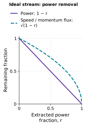
A DEFINED STREAM LEDGER / NOT A COMPLETE ENGINE
Picture a fast stream leaving a nozzle. A generator can take some of the stream's motion, but that slows the stream and reduces its push. Some electricity is lost in conversion; equipment needs power; an accelerator can return only part of the remaining electricity as extra jet speed. Count every part before calling the idea a gain.
This example begins after fuel has burned, at the rear engine opening where the exhaust leaves. It holds exhaust mass flow, incoming speed, and the pressure-thrust term fixed. It is deliberately narrower than a complete aircraft or scramjet balance. It connects kinetic-energy extraction, generator loss, auxiliary demand, electrical export, accelerator return, exhaust speed, and momentum thrust in one consistent example. It tracks only jet motion energy: heat stored in the hot gas or engine is not collected in this model. It does not reuse the separate 515.7 kJ/kg inlet calculation: that is energy transferred from motion to the air pressure-and-temperature state during ideal inlet slowing, not electricity available to harvest.
Illustrative output.
Energy check: 2,000.0 kW accounted for from 2,000.0 kW.
Pstream,0 = ½ṁVe,0² · Premoved = fPstream,0 · Pelectric = ηgPremoved
Preturned = ηas max(0, Pelectric − Paux) · Ve,1 = √(Ve,0² − 2 × 1000(Premoved − Preturned)/ṁ)
Fmomentum = ṁ(Ve − V∞) · ΔF = F1 − F0
Read the signs and boundary: both speeds are positive downstream flow-speed magnitudes at the inlet and exit stations, expressed in one steady, instantaneous vehicle-fixed frame. This simple convention reports the forward-thrust contribution on the vehicle; a negative change means that contribution is smaller than baseline. The same mass flow is imposed in both cases: fuel addition, bleed, inlet capture/spillage changes and flow-rate changes are omitted. The nozzle pressure term is set to zero for the displayed example and held unchanged for the comparison by assumption, not because the energy equation guarantees it.
For an engine, NASA’s general thrust relation also includes the nozzle pressure term, which this example holds fixed: NASA Glenn · Thrust force.
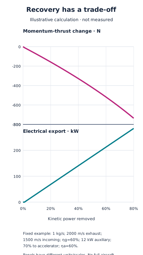
Worked reference: ṁ = 1.0 kg/s; baseline exhaust speed Ve,0 = 2,000 m/s; incoming air speed V∞ = 1,500 m/s, all in the same steady vehicle-fixed inertial frame. Baseline kinetic power is 2,000 kW and the baseline momentum-only thrust is 500 N with the pressure term set to zero. Slider values for removal fraction, efficiencies, auxiliary load and accelerator share are chosen teaching assumptions, not measurements or a proposed engine specification. The accelerator share is applied after the auxiliary demand; any remaining bus power is shown as export. The unmet auxiliary portion is reported if generation is too small.
Here “power returned” is an assumed lumped conversion: a chosen share of generator electricity is treated as directed kinetic power added to this same stream. The model does not calculate electrode geometry, electrical conductivity, current closure, magnetic-field generation or self-excitation, or the electromagnetic force along the flow. For this simplified account, Pstream,1 + generator loss + served auxiliary power + accelerator loss + electrical export = Pstream,0. The generator and accelerator losses are treated as heat leaving this bookkeeping boundary; where that heat would go, or whether it later warms the gas or vehicle, is not calculated. So this is not a complete engine thermodynamic balance. The force comparison includes only ṁ(Ve−V∞) at the two stated stations with an unchanged pressure term. It does not calculate inlet capture or spillage, pressure drag, total-pressure loss, shocks, heat transfer, combustion matching, electrical conductivity, magnet mass, cooling, vehicle drag, added mass, mission range or fuel use. The displayed absolute thrust assumes a zero pressure-thrust term; only the momentum contribution and its change are calculated. The MHD generator-before-combustor bypass shown above is a distinct analyzed layout; this post-combustor stream ledger does not claim to reproduce that layout or any tested complete loop.
Thus a negative momentum-thrust change here is a consequence of the defined arithmetic, while the total change in aircraft performance remains unknown. A complete evaluation needs a coupled cycle and vehicle model supported by evidence for every component.
Separate models: the hover and ideal carried-propellant exercises below teach momentum and power. Neither simulates this hypersonic air-breathing vehicle.
01 / ATMOSPHERIC OBSERVATION
Design brief: hold a camera or environmental sensor in still air. The comparison assigns a total mass of 5 kg, including every component.

The importance of rotor–body and wake interactions is supported by NASA's multirotor airflow study. That study does not validate this particular sketch.
| Four-rotor layout | Total disk area | Each rotor diameter | Ideal induced power |
|---|---|---|---|
| Smaller disks | 1 m² | 0.56 m | 219 W |
| Larger disks, illustrated | 4 m² | 1.13 m | 110 W |
Equal loading and negligible rotor interaction are assumed in this calculation. These are diameters of each of four rotors, not the single disk in the earlier example. Real electrical power is higher. If the larger structure adds mass, the comparison must be recalculated.
Change mass and total area in the hover model →
Specify payload, wind, flight duration and footprint. Then size the blades, motors, structure and battery together; check clearances, noise, airflow interference, control and failure behaviour. Measure electrical power at matched payload and conditions. No claim is made that the illustrated large layout can actually be built at 5 kg.
Useful outcome: keeping a sensor at an observation point. A future improvement would be longer observation with the same payload, confirmed by measured power, noise and stability—not inferred from disk area alone.
02 / SOLAR-ELECTRIC CRUISE
Design brief: change orbit gradually after launch. Sunlight provides energy; carried xenon provides matter to eject. This is not an Earth launch vehicle.

These choices draw on the Psyche mission design study, NASA plume-interaction research and NASA thermal-control guidance. The illustrated arrangement is an educational synthesis, not a reconstruction of those missions.
The instruments, electronics and control systems also need electricity. Thruster power is what remains after those demands and operating margins. Sunlight weakens farther from the Sun; adding solar panels adds mass and packaging demands.
Explore why faster exhaust demands more power →
The 1 N slider is a separate arithmetic example, not a performance specification for this spacecraft. Gridded-ion and Hall thrusters are different technologies; neither is selected or sized by this outer-layout drawing.
Choose the destination and travel time, then calculate trajectory, total mass, solar-array area, power electronics, propellant capacity, heat rejection, thruster lifetime and launch packaging. Test the plume and pointing envelope. A high exhaust speed alone does not prove a shorter or lighter mission.
Useful outcome: visiting multiple destinations with a limited propellant budget. Dawn explored Vesta and Ceres using ion propulsion. A future improvement must be demonstrated across thrust, input power, lifetime and total system mass together.
START HERE / WHAT PUSHES BACK?
Propulsion changes a machine's motion through a push, called thrust. Hovering also needs a push to balance weight. Ask what exchanges momentum with the machine and where its energy comes from.
A drone accelerates air downward; the air pushes it upward. This can hold a camera over a fixed location. Total mass, swept area and losses affect power demand. A rotor cannot provide this kind of lift in a vacuum.
A rocket accelerates carried propellant away. It does not need to push against the atmosphere. Chemical and electric engines supply energy differently; both account for expelled matter. The ideal exhaust exercise compares one trade-off, not complete engines.
A current can experience force in an external magnetic field. Include the complete circuit and identify the field source or surrounding medium exchanging momentum. Force on one wire is not automatically thrust on a vehicle.
Thrust is force in newtons (N). Power is energy transferred each second in watts (W). Propellant flow is the mass ejected each second in kilograms per second (kg/s).

A PRACTICAL QUESTION / HOLDING A CAMERA STILL
A complete 5 kg camera platform hovering in still air of density 1.225 kg/m³ needs about 219 W of ideal induced power with 1 m² of swept disk area, or 110 W with 4 m². Both need the same 49 N upward force. Spreading the push over more air reduces the required change in air speed.
For one circular disk, those areas mean diameters of about 1.13 m and 2.26 m. A larger structure may add mass: include camera, battery, motors, blades and frame. These values exclude motor and aerodynamic losses and do not predict battery life or select a safe aircraft design.

01 / MOVE MORE AIR, MORE SLOWLY
An ideal rotor spreads its downward push over a disk of air. A larger disk can move more air at a lower speed for the same upward force, reducing the ideal power requirement. Disk area means the swept circular area, not the material area of the blades.
Density is an independent illustrative input, not an altitude calculation.
Reference: 5 kg, 1 m² and 1.225 kg/m³ give 49.033 N and 219.36 W of ideal induced power. Quadrupling area halves that power. Doubling supported mass multiplies it by about 2.83.
T = mg · vᵢ = √(T/(2ρA)) · ṁ = ρAvᵢ · vwake = 2vᵢ · Pᵢ = Tvᵢ
The outgoing momentum flow is ṁvwake = T. The outgoing kinetic-energy flow is ½ṁvwake² = Pᵢ. Air at the disk moves at half the far-wake speed in this ideal model. Mixing up those two speeds breaks the balance.
Assumptions: steady, incompressible, uniform open actuator disk in initially still air, hovering away from surfaces. Gravity is 9.80665 m/s². Blade drag, swirl, motor/controller losses and airframe effects are omitted. Structural design and added-mass estimation are not calculated; the entered mass must include the whole vehicle. This is an ideal reference within those assumptions, not a universal minimum for buoyancy, ducts or ground-effect machines.
Actual hardware needs additional power. An efficiency, endurance, payload or flight-safety claim cannot be inferred from this model. Multiple disk areas may be summed only for suitably noninteracting disks with equal loading; overlapping rotors are different.
SPACE / AN IDEAL EXHAUST COMPARISON
Hold thrust at an assigned 1 N. Faster exhaust carries more momentum per kilogram, so less propellant is needed each second. But each kilogram carries more kinetic energy. This instantaneous vehicle-frame model assumes carried propellant and a pressure-matched jet; it is not atmospheric ionic wind or a complete engine.
At 1,000 m/s: 1 g/s and 500 W. At 10,000 m/s: 0.1 g/s and 5,000 W, for the same 1 N.
T = mass flow × exhaust speed; jet power = ½ × mass flow × speed² = ½Tv. Pressure thrust is set to zero. The calculation omits plume divergence, undirected thermal energy, ionization, power-system losses and mass, structural limits and trajectory evolution. It predicts neither engine efficiency nor mission endurance. A rocket can work in vacuum because it ejects matter, not because it pushes against air.
The study's dashed input-power curve divides jet power by an assigned efficiency of 0.60. This is a hypothetical comparison, not a measured engine efficiency. The controls show only directed jet power.
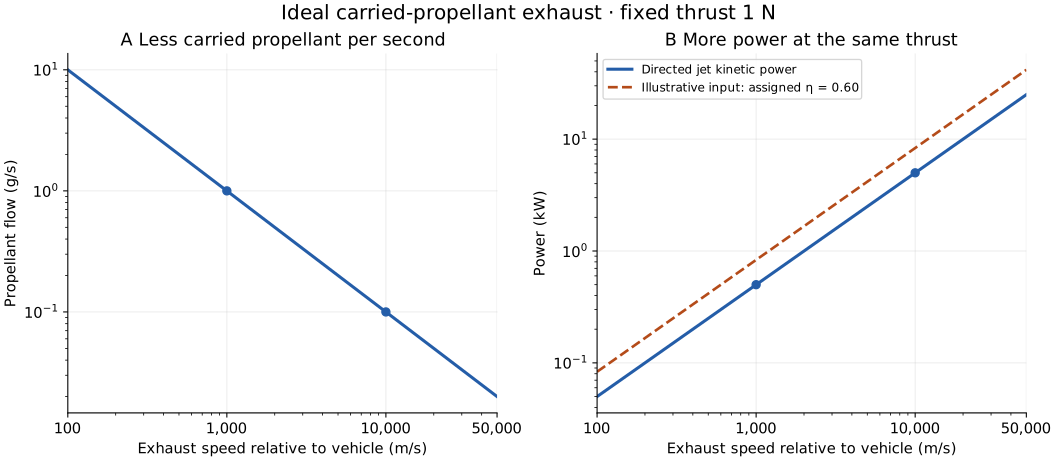
| Speed | Flow | Jet power |
|---|---|---|
| 1,000 m/s | 1 g/s | 500 W |
| 10,000 m/s | 0.1 g/s | 5,000 W |
Study data CSV · Figure PDF · Methods and limits · Reproduction script · Phone layout figure · SVG
02 / FOLLOW THE REACTION PARTNER
A rotor transfers momentum to air. Electroaerodynamic propulsion uses electric forces on ions and collisions with neutral air. No moving propeller does not mean no moving matter. Demonstrated fixed-wing ionic-wind flight is not evidence of hover for an unspecified machine.
Electrical energy accelerates ionized propellant outward; the spacecraft recoils. A neutralizer prevents charge buildup. Electricity supplies energy, while propellant carries momentum.
A current can interact with an externally produced magnetic field. Include the field source, return circuit and electromagnetic momentum in the overall accounting. Internal attraction between carried parts does not create sustained thrust of an isolated whole.
For a simple pressure-matched exhaust, thrust is mass flow times exhaust speed. Its kinetic power is one half of thrust times exhaust speed. Higher exhaust speed saves propellant for a given thrust but demands more jet power. Real electrical power depends on losses; this is not a complete engine design.
A MEASURED SPACE-PROPULSION COMPARISON
Simple version: A Hall thruster pushes a spacecraft forward by sending charged xenon backward. Electricity supplies the energy; the spacecraft carries the xenon. It does not scoop air.
A NASA team tested an engineering Hall-thruster unit under vacuum at four reference settings. Between 6.25 and 12.50 kW of discharge power, the tested ETU-2 rose from 397 to 611 mN of thrust, from 1,968 to 2,826 seconds of specific impulse, and from 60.5% to 67.4% reported total efficiency. NASA compared it with earlier Technology Demonstration Units (TDU); the slide says the results matched within the empirical uncertainty. This is test-article evidence, not flight performance. NASA presentation record · 2021 presentation PDF.
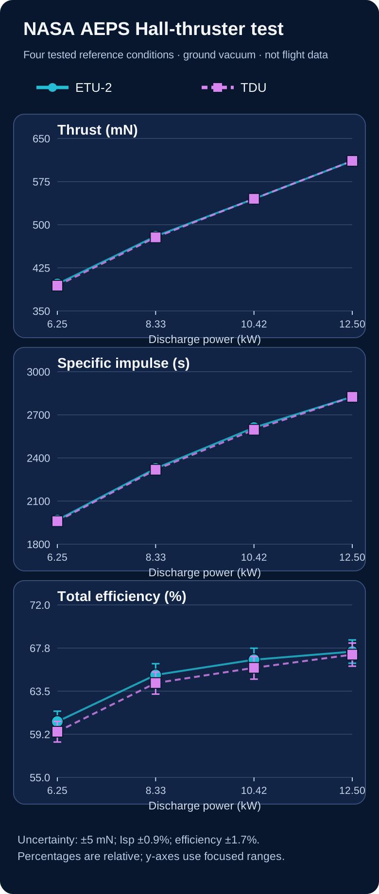
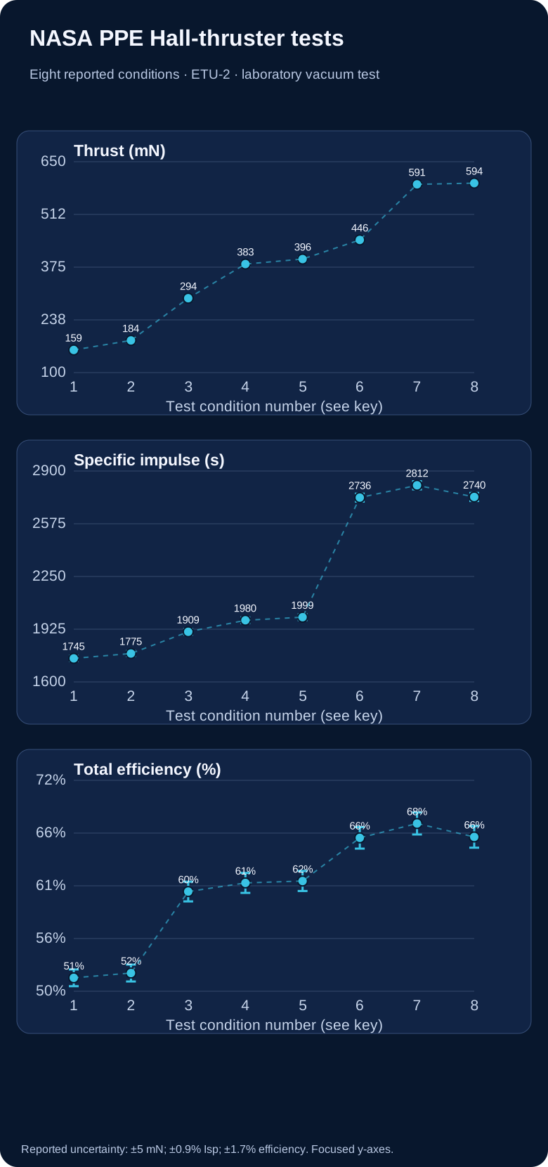
| Source condition | Thrust (mN) | Specific impulse (s) | Total efficiency (%) |
|---|---|---|---|
| 300 V / 2.60 kW | 159 | 1,745 | 51.4 |
| 300 V / 3.00 kW | 184 | 1,775 | 51.9 |
| 300 V / 4.50 kW | 294 | 1,909 | 60.4 |
| 300 V / 6.00 kW | 383 | 1,980 | 61.3 |
| 300 V / 6.25 kW | 396 | 1,999 | 61.5 |
| 600 V / 9.00 kW | 446 | 2,736 | 66.0 |
| 600 V / 12.00 kW | 591 | 2,812 | 67.5 |
| 600 V / 12.00 kW / 14% | 594 | 2,740 | 66.1 |
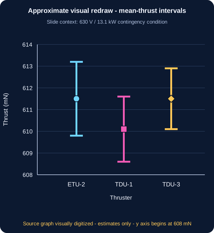
What the study supports: a NASA engineering-thruster ground-test comparison over the stated conditions. It does not test hypersonic atmospheric inlets or an MHD energy-bypass propulsion loop.
| Discharge power | Thrust ETU-2 / TDU (mN) | Specific impulse ETU-2 / TDU (s) | Total efficiency ETU-2 / TDU (%) |
|---|---|---|---|
| 6.25 kW | 397 / 394 | 1,968 / 1,960 | 60.5 / 59.5 |
| 8.33 kW | 480 / 478 | 2,327 / 2,318 | 65.1 / 64.3 |
| 10.42 kW | 545 / 545 | 2,611 / 2,596 | 66.6 / 65.8 |
| 12.50 kW | 611 / 611 | 2,826 / 2,825 | 67.4 / 67.1 |
The NASA presentation reports a 2019–2021 engineering-unit test campaign at Glenn Research Center. Power and propellant were supplied by calibrated laboratory systems; thrust was measured with an inverted-pendulum stand. The reported nominal operating pressure at the 12.5 kW point was about 4.5 µTorr in NASA's VF-5 vacuum facility. The 2021 results slide reports ±5 mN thrust, ±0.9% specific impulse and ±1.7% total efficiency uncertainty. Those are source-reported uncertainties, not error bars independently recomputed here.
The source's study goal included supporting an application of the Advanced Electric Propulsion System to Gateway's Power and Propulsion Element. That is the purpose stated for this test program, not proof that these test results constitute a delivered or flight-qualified spacecraft system.
Program status, checked 29 September 2026: NASA’s current SR-1 Freedom mission page lists the Power and Propulsion Element as the spacecraft bus, with an AEPS 12-kW Hall thruster, and targets launch in late 2028. This is a stated mission plan, not evidence of completed spacecraft integration or flight. NASA’s AEPS program overview, last modified 21 September 2026, says qualification tests on two thruster units are under way and expected to finish in 2027. The measurements here remain ground-test evidence. NASA SR-1 Freedom mission plan · NASA AEPS qualification update.
This comparison is about in-space electric propulsion with carried propellant and supplied electrical power. The separate hypersonic inlet/MHD idea concerns a conducting atmospheric flow, different device boundaries and substantial pressure, ionization, field and thermal losses. This NASA Hall-thruster test gives no evidence that inlet flow energy can be recovered or that an MHD bypass improves an atmospheric vehicle.
Download the transcribed measurements (CSV) · Extraction and plotting method · Reproduce reference-condition graphs (Python).
Why this kind of evidence matters: mission designers can compare a real measured thrust–power–propellant trade-off before deciding whether a technology fits a spacecraft task. The measurements inform a bounded technology comparison; mission usefulness still depends on spacecraft power, propellant, duration and trajectory.
SPACE PROPULSION · MEASURED TRADE-OFFS
Simple version: A spacecraft carries propellant and uses electricity to send a little of it backwards. Depending on the engine, that propellant can start as a gas, liquid or solid. That gives the spacecraft a gentle push forwards. The push can be tiny, but it can keep working for a very long time. The spacecraft does not scoop air, and it still needs a power source and propellant.
Specific impulse (Isp) is a way to compare how efficiently a thruster turns propellant into push. In a simple ideal model, more Isp means faster exhaust and less propellant for the same push, but the fast exhaust carries more kinetic energy. The unit “seconds” is a comparison unit, not the time the engine must run.
Imagine the same 1 newton push from two imaginary thrusters. Using exhaust speed = Isp × 9.80665 m/s², mass flow = thrust ÷ exhaust speed, and jet power = ½ × thrust × exhaust speed:
| Assumed Isp | Equivalent exhaust speed | Propellant flow | Ideal jet power |
|---|---|---|---|
| 2,000 s | 19.6 km/s | 0.051 g/s | 9.8 kW |
| 4,000 s | 39.2 km/s | 0.025 g/s | 19.6 kW |
The faster case uses about half as much propellant each second, but needs about twice the ideal jet power for that same 1 N. A real power supply needs more electrical power because of conversion losses and other spacecraft loads. These chosen settings describe a teaching comparison, not a named thruster or flight test.
A RECENT MEASURED PLASMA-THRUSTER STUDY
For a five-year-old: Picture a tiny electric push that sends a puff of gas backwards. Researchers tested how the amount of supplied gas entering the discharge changes the push.
Horstman, Woodley and Underwood studied a laboratory gas-fed pulsed plasma accelerator using air. Its valve, gas-conditioning and coaxial-electrode stages fed a short capacitor-bank discharge. A high-speed camera followed the glowing plume front; a separate calibrated pendulum measured each pulse’s impulse.
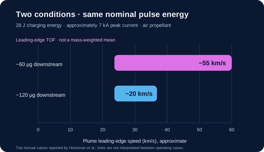
| Downstream air mass | Leading-edge TOF speed | Observed mode |
|---|---|---|
| ~60 μg | ~55 km/s | Weakly unstable magneto-deflagration |
| ~120 μg | ~20 km/s | Magneto-detonation |
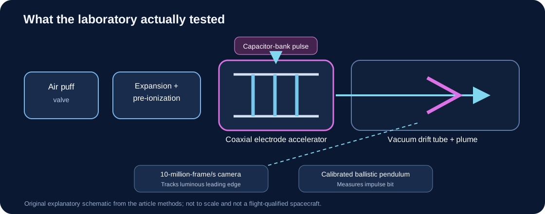
What is genuinely useful: the study maps how pulse current and initial gas loading can move the accelerator between a shock-like “magneto-detonation” mode, a smoother “magneto-deflagration” mode, and an unstable region. The paper reports 26 operating combinations. This gives researchers a practical way to think about controlling how much gas a pulsed electric engine actually catches in its plasma push.
The important limit: high leading-edge speed does not by itself show high useful thrust or total-system efficiency. At about 15 μg and 40 J, the authors say the device begins to run gas-starved and electrode material can be eroded and added to the plume. Very-low-mass, high-specific-impulse values therefore need the electrode-life and mass-accounting caveat.
Source-text discrepancy to verify: the article’s abstract reports propellant utilization rising from 5% to 35% as downstream mass falls from 70 to 10 μg. Its detailed results instead report 10% to 35% over 70 to 15 μg; the Figure 11 caption also places the sharp rise near 15 μg and says onset of electrode ablation may affect it. We preserve both published summaries rather than choosing one. The article does not provide machine-readable point data here to resolve the mismatch, and the lowest-mass region needs separate electrode-material accounting.
A conditional arithmetic check: Section 4.2 reports an impulse-bit range of 334 to 140 μN·s while downstream mass ranges from 70 to 15 μg. If we provisionally pair those range endpoints in the stated order and use the paper’s equation, Isp = impulse bit ÷ (g₀ × downstream mass), the calculated values are about 486.55 s and 951.74 s. These fall within the article’s broader 100–2,000 s range, but the paper does not publish an endpoint-by-endpoint numerical table, so this pairing is a check rather than recovered point data. In base twelve the same approximate values are 346.672B20A9₁₂ s and 673.89A38488₁₂ s; this is only a notation conversion, not added precision. We do not combine these values with the ~55 km/s result from Figure 10, which used a different 28 J / ~7 kA condition; Figure 11 uses 40 J / 8 kA.
Possible human benefit, still a research prospect: a future air-breathing electric system might collect thin upper-atmosphere gas instead of carrying all of its propellant, potentially helping a satellite stay in very low orbit. This experiment did not demonstrate atmospheric capture, a complete collector-to-thruster loop, orbit maintenance, spacecraft lifetime, or a flight-ready vehicle. The test used supplied air in a vacuum chamber.
Two approximate source values · CSV · Methods, provenance and limits · JSON. The paper’s supporting data are not supplied as a machine-readable dataset in this figure record; these two values are copied from its prose, not digitized point-by-point from the graph.
In space, electric propulsion converts electrical energy into the motion of expelled propellant. The electricity has usually come from solar panels; a reactor or another source is possible in principle. “Electric propulsion” covers several different kinds of engine, so no single number describes them all. NASA’s 2026 small-spacecraft survey separates these technologies and warns that its ranges summarize the devices it reviewed—they are not universal limits.
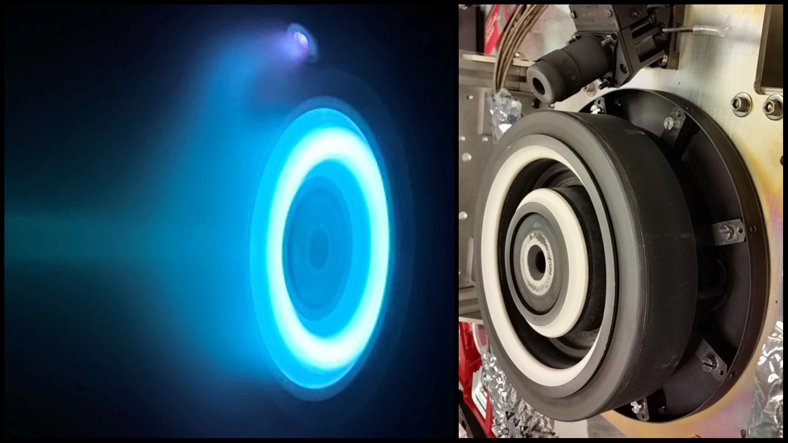
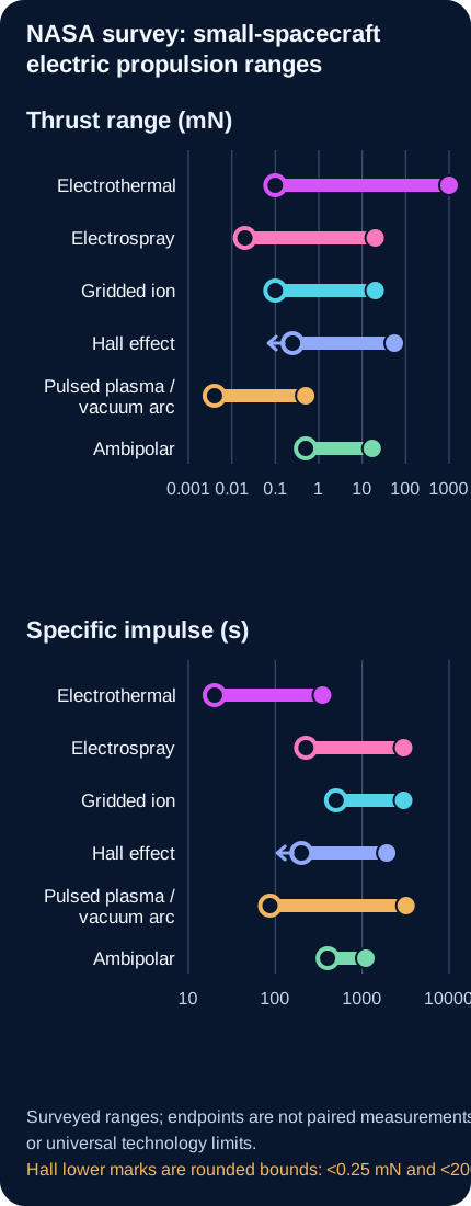
NASA’s chart is a useful survey of selected small-spacecraft devices, not a set of independently tested technology limits. The entries mix manufacturer specifications, nominal values, component and integrated-system data, reported flight demonstrations, and different operating conditions. The thrust and specific-impulse extremes are not necessarily from the same device or operating point.
The low entries trace to an AIS SWAG1-PQ catalog listing. The 1 N upper thrust is the marketed upper bound for the Benchmark Starling Ardent family; the source does not establish that 1 N as an independently demonstrated point. The 350 s value is an EPL APS500 manufacturer specification. AIS product listing · Starling Ardent data sheet · EPL resistojet range.
NASA Table 4-1’s 20 μN is the lowest nominal survey entry, not the minimum operating capability. The 2026 PDF Table 4-8 lists Busek CMNT (4× heads), “4 × 20” under [μN]. The primary 2017 ST7 flight-performance paper says a CMTA has four heads, each individually throttleable from 5 to 30 μN (PDF pp. 4–5), supporting 20 μN per head as the 2026 nominal-row reading. Four heads at that point sum arithmetically to 80 μN if all operate together; the survey row does not establish that simultaneous flight condition. NASA’s live HTML says [mN], apparently a factor-1000 label/version error relative to the PDF and flight report. NASA separately documents the integrated LISA Pathfinder flight demonstration. The 20 mN maximum and 3000 s maximum trace to different Enpulsion product entries, not one paired operating point or class limit. NASA 2026 PDF, Tables 4-1 and 4-8 · NASA live HTML, Table 4-8 · NASA LISA Pathfinder flight record · Enpulsion current product data sheets.
NASA’s summary Table 4-1 reports 0.1 mN and 500 s as category lower bounds. This audit did not identify either lower bound in a named-device row of detailed Table 4-9; treat them as summary-table ranges, not verified device capability limits or a paired operating point. At the high end, the T5 source lists capability or throttle bounds around 20 mN and 3000 s; these should not be read as one measured endpoint pair. T5 performance source cited by NASA · ESA’s GOCE engine record.
The NASA survey lists the MUSIC-SI low values as “less than 0.25 mN” and “less than 200 s,” but its summary turns those into exact-looking minima. MaSMi’s 55 mN and 1920 s are survey entries; a published 2019 characterization reports different peak values, 68.6 mN and 1940 s at 1 kW. Configuration differences need resolution, so neither figure should be treated as a universal Hall-thruster ceiling. NASA chapter PDF, Table 4-10 · MaSMi published characterization.
The 4 μN lower thrust is NASA’s rounding of an ND-15 value reconstructed from the manufacturer’s 45 μN·s impulse bit multiplied by its 83 mHz maximum frequency. The data sheet does not state that both occur together. CU Aerospace lists 0.50 mN at 96 W and up to 3200 s for FPPT-1.7; AIS lists 87 s for VAT1-PQ. These are manufacturer specifications, not a common independent test. NASA’s 2026 PDF Table 4-11 gives the Neumann ND-15 as 3.75 and CU Aerospace FPPT-1.7 as 500 under [μN]; the live HTML shows the same numbers under [mN]. The PDF summary Table 4-1 gives 4–500 μN, consistent with the detailed PDF after rounding 3.75 to 4. The HTML unit therefore appears mislabeled by a factor of 1,000; this graph follows the PDF and summary units. A header-only cross-check of NASA’s detailed electric-propulsion Tables 4-7 through 4-12 finds unit-label mismatches in Tables 4-8 and 4-11; the thrust units in Tables 4-7, 4-9, 4-10 and 4-12 match across editions. This cross-check concerns unit headers only, not every table cell. NASA 2026 PDF, Tables 4-1 and 4-11 (printed pp. 66 and 116) · NASA current HTML Table 4-11. Neumann ND-15 data sheet · CU Aerospace FPPT data sheet · AIS VAT1-PQ product page.
T4i lists 0.55 mN at 50 W for its integrated REGULUS-50 system. NASA’s 2022 survey lists the Miles M1.4 (water) at 2.8 mN, 1,340 s, 3.3 kN-s and <11.5 W. The 2024 and 2026 NASA surveys list 17.2 mN and 6 W, but give no specific-impulse or total-impulse value; listed mass and dimensions also differ. These are survey entries, not matched primary test records. Test conditions and configuration equivalence remain unresolved, so the higher later thrust entry is not evidence of a measured 6.1-fold performance improvement. This bounded audit did not trace an independent primary thrust test. RocketStar · FireStar Foundation M1.4 specs · NASA 2022 survey · NASA 2024 survey · NASA 2026 survey. The 400–1100 s values are nominal entries for different Maxwell configurations and propellants; their exact complete-system test endpoints remain unconfirmed. T4i REGULUS-50 · RocketStar · FireStar Foundation M1.4 specs · NASA 2022 survey.
Open the complete endpoint-by-endpoint ledger, status labels, and limits. This is a bounded audit, not a device test campaign or exhaustive literature review.
| Technology | Thrust range | Specific-impulse range |
|---|---|---|
| Electrothermal | 0.1 mN–1 N | 20–350 s |
| Electrospray | 20 μN–20 mN | 225–3,000 s |
| Gridded ion | 0.1–20 mN | 500–3,000 s |
| Hall effect | 0.25–55 mN | 200–1,920 s |
| Pulsed plasma / vacuum arc | 4–500 μN | 87–3,200 s |
| Ambipolar | 0.5–17 mN | 400–1,100 s |
These short guides cover all six families in NASA’s small-spacecraft table. Their reported performance ranges differ by device, and some entries describe components rather than complete propulsion systems. Examples show an application or a test status; they do not mean every model in a family is flight-proven.
Electricity heats a gas; a nozzle sends the hot gas backwards. Resistojets heat a surface, arcjets heat an ionized gas, and other devices heat the gas without electrodes in the flow. This approach can use different propellants, including water in some systems. Hot materials and heat flowing back into the spacecraft constrain the design. On SPHERE-1 EYE, the team reported operating all four water-resistojet nozzles in orbit and estimated thrust of 6.1–7.2 mN; its public abstract does not establish direct force measurement. Ground tests separately reported 2.7 mN and 60 s specific impulse. Authors’ 2023 conference abstract (SSC23-VI-02) · Operator’s telemetry-based confirmation.
The engine makes ions, then electric fields pull them through fine grids to form a fast exhaust. A downstream neutralizer normally adds electrons to the beam, helping keep the spacecraft from accumulating charge. These engines can reach high specific impulse, so they can use propellant sparingly over a long mission. The trade-offs include low thrust for the electrical power, high-voltage equipment and slow erosion of the grids.
A magnetic field helps hold electrons in the engine while an electric field accelerates positive ions outwards; a separate neutralizer balances the exhaust charge. NASA’s comparison says Hall engines usually provide more thrust for a given power than gridded-ion engines, while gridded-ion engines can reach higher specific impulse. In the small-spacecraft survey, Hall engines occupy a compromise region between thrust and specific impulse; the right choice still depends on the mission and full spacecraft system.
A strong electric field pulls charged ions or tiny charged droplets from a liquid propellant. These very small pushes can be finely controlled, making electrosprays useful for precise pointing or gentle orbit adjustments. NASA’s 2026 survey identifies plume impingement and possible surface contamination as spacecraft-integration risks, not a measured universal effect. On UWE-4, engineers measured a change in spacecraft rotation during a NanoFEEP firing; the authors inferred that part of the plume was reaching an antenna and adding torque, but they did not measure chemical deposits. Separately, LISA Pathfinder accumulated more than 2,400 colloid-thruster operating hours; a suspected propellant bridge inside one thruster’s electrodes is a different issue, not evidence of external plume contamination. NASA survey, §4.6.2 · UWE-4 conference paper record · LISA Pathfinder flight paper, Appendix A.2.
A small electrical discharge releases and accelerates a brief puff of plasma from solid propellant. The tiny pulses can steer a small satellite accurately, and the compact units can suit spacecraft with modest power. The energy-storage hardware adds mass; heating, wear and changing propellant surfaces affect efficiency and lifetime. A 2026 Small Satellite Conference presentation by the DUPLEX team reports initial flight-test data for its fiber-fed pulsed-plasma thruster and says operations continue to gather on-orbit data. This is early evidence for that particular system, not broad validation of every pulsed-plasma or vacuum-arc design.
DUPLEX team · 2026 initial flight-test presentation · NASA · system description and deployment
A radio-frequency field makes a gas into plasma. Electrons escape more easily than heavier ions, and the resulting electric field helps push ions out. The plume can remain electrically balanced without a separate neutralizer, but the radio-frequency power, heat, and interference with spacecraft electronics must be managed. NASA’s survey notes that the manufacturer reported an on-orbit demonstration of its Maxwell Block 2 system; this is a technology demonstration, not proof that every ambipolar design is ready for any mission.
How to read “specific impulse”: it measures thrust per unit of propellant weight expelled each second and is usually reported in seconds. Higher specific impulse can mean less propellant for the same total change in spacecraft velocity, but it does not mean stronger immediate acceleration. The spacecraft’s acceleration also depends on its mass. Electric engines generally trade lower thrust for high exhaust velocity and lower propellant use; they still need sustained electrical power and often long operating times. NASA notes that electric systems in its survey may need hundreds or thousands of hours to build up the same total impulse that a chemical engine can deliver in seconds or minutes. These ranges do not include every spacecraft-level power-source mass or mission constraint.
NASA describes Space Reactor-1 Freedom as a future mission targeting launch in late 2028. Its mission page separately lists a 20 kWe closed-Brayton power-conversion system, a spacecraft-bus Power and Propulsion Element “generating 48 kilowatts of electrical power,” and a 12-kW Advanced Electric Propulsion System Hall thruster. The public page does not show one operating-point power chain that reconciles those entries, so they remain separate here; they must not be added or treated as a closed energy balance. The mission is planned, not flight evidence.
A separate NASA technical overview describes the 12-kW AEPS Hall thruster for Gateway’s Power and Propulsion Element. That reference provides context for the thruster class; it does not resolve the SR-1 power figures. NASA’s SR-1 Freedom mission and power page · NASA’s AEPS technical overview · NASA’s 2024 Gateway propulsion-system status.
For a five-year-old: Imagine a tiny fan gently pushing a very heavy toy spaceship. It does not jump forward; it keeps nudging for many days. The longer it nudges, the more the spacecraft’s speed changes.
What NASA measured: In a vacuum-chamber test of the AEPS Hall thruster, one operating point produced 594 mN thrust at 12 kW discharge power and 2,740 s specific impulse. These are paired laboratory values, not flight measurements. The source table gives uncertainties of ±5 mN in thrust and ±0.9% in specific impulse; the reported total efficiency is 66.1% ±1.7%.
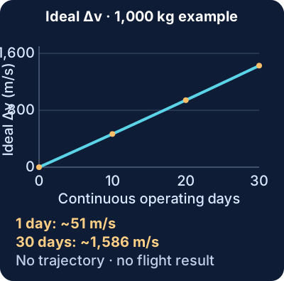
| Quantity | Value | Evidence status |
|---|---|---|
| Thruster thrust | 594 ± 5 mN | NASA ground-test measurement |
| Specific impulse | 2,740 s (±0.9%) | Same reported operating point |
| Discharge power | 12 kW | Same ground-test operating point |
| Initial acceleration at 1,000 kg | 0.000594 m/s² (0.594 mm/s²) | Calculated from measured thrust ÷ assumed mass |
| After one continuous day | about 51.4 m/s ideal Δv; about 1.91 kg propellant used | Calculated using measured thrust/Isp and ideal rocket equation |
| After 30 continuous days | about 1,586 m/s ideal Δv; about 57.3 kg propellant used | Hypothetical calculation; constant operating point |
At this thruster’s tested power and thrust, the acceleration of the assumed 1,000 kg spacecraft is tiny; this engine is intended for gradual in-space changes, not to launch its spacecraft from the ground. Thrust is a force; acceleration depends on spacecraft mass. Specific impulse helps estimate exhaust speed and propellant flow. Here, 594 mN divided by an assumed 1,000 kg gives the initial acceleration. The ideal rocket equation accounts for the spacecraft getting lighter as it uses propellant.
Effective exhaust speed is ve = Ispg0 = 2,740 × 9.80665 ≈ 26,870 m/s. Propellant flow is estimated from the measured thrust: ṁ = F/ve ≈ 2.21 × 10⁻⁵ kg/s. For each elapsed time, propellant used is ṁt and ideal Δv = ve ln(m0/m0−ṁt), with m0 = 1,000 kg. The plotted values are reproduced from the paired point in NASA’s source table; see its slide 13 and the retained CSV/methods files.
The 1,000 kg spacecraft, continuous operation and constant thruster point are teaching assumptions. The plot omits array and power-system mass, changing solar power, thermal limits, engine wear, thrust direction, orbit geometry, gravity, eclipse time, coast periods and navigation. Therefore the Δv values are not an achievable mission promise. The test’s efficiency and discharge power describe the thruster; they do not establish a complete spacecraft power-system performance.
Source: Frieman et al., NASA Glenn, “Performance of the 12.5-kW Advanced Electric Propulsion System Engineering Test Unit Hall Thruster,” 2021 JANNAF presentation, slide 13 (NTRS 20210015735). NASA source record and presentation.
Change one assumption and see how electrical power and exhaust speed trade thrust against propellant. This is an idealized teaching calculation, not a trajectory or spacecraft-performance prediction.
Very small positive results use scientific notation so they are not mistaken for zero. Burns under ten minutes are shown in seconds; burns from ten minutes to one hour are shown in minutes. The dry-mass setting is the reserve stop line; it changes how much propellant is available, not the thrust of the engine.
The full selected burn fits within the entered propellant allowance.
It uses effective exhaust speed ve = specific impulse × standard gravity, steady thrust F = 2ηP/ve, propellant flow ṁ = F/ve, and the ideal rocket equation Δv = ve ln(minitial/mfinal). Here η means the entered fraction of thruster electrical input converted to directed exhaust kinetic power. It stops at the entered dry-mass reserve.
The default values are illustrative inputs, not measurements from a named engine. The model assumes constant delivered power, efficiency and specific impulse. It omits the mass and changing output of solar arrays or another power source, power-system losses not included in η, engine lifetime, thermal limits, thrust vectoring, gravity, trajectory, coasting and operational constraints. NASA’s device ranges above are separate min-to-max envelopes, not paired operating points. A realistic mission needs a coupled spacecraft and trajectory analysis.
Efficiency and specific impulse can be changed independently in this teaching model. A real thruster does not necessarily achieve every combination of the two; compare measured, paired operating points before assessing a particular engine.
NASA’s Dawn spacecraft used one ion engine at a time to enter orbit around both Vesta and Ceres. It carried 425 kg of xenon; each engine could produce up to 91 mN, and the mission accumulated more than 2,000 days of thrust. The long, gentle push enabled Dawn’s planned two-world orbit mission, which NASA says would have been impossible without ion propulsion.
ESA’s SMART-1 used a single solar-electric Hall thruster for a gradual, spiralling trip from Earth orbit to the Moon. Its propulsion system produced about 70 mN while using 82 kg of xenon. The engine helped enlarge the spacecraft’s Earth orbit, capture it at the Moon and adjust its lunar orbit. The long transfer took about 13 months—a real mission showing the value of a small, steady push.
ESA engine specifications · ESA completed-mission operations record
NASA’s mission summary lists up to 240 mN for the active unit. A peer-reviewed report reconstructed higher thrust during the 2023–24 initial checkout: Thruster B reached 278.8 ± 0.4 mN (3σ) at the end of a 4.5 kW calibration burn. This was inferred from Deep Space Network radio tracking, not measured with a force sensor. During a separate week-long systems test, the reconstructed value fell from approximately 278 mN to 257 mN about two days later (an approximately 8% decline); the team noted early-life burn-in and possible plasma-mode changes, while the exact timing was uncertain by about a day. These are specific checkout episodes, not a fixed rating or lifetime guarantee. Psyche has four Hall thrusters installed, uses one at a time, and carries as much as 1,085 kg of xenon. Its solar arrays can produce 21 kW near Earth, compared with 2.3–3.4 kW near the asteroid, so available power changes along the journey.
NASA spacecraft summary · Peer-reviewed flight report: Table 1 and Fig. 16
ESA reports that this commercial communications satellite used electric thrusters to climb to its equatorial working orbit about 35,800 km above Earth, reaching it roughly four months after launch. It then used electric propulsion for station-keeping. The slow climb traded transfer time for low propellant use; Eutelsat reports service including broadcast and in-flight broadband across the Asia-Pacific.
ESA orbit-raising and station-keeping record · Eutelsat service announcement
Simple version: Electric thrusters do different jobs. Some change an orbit, some cancel a tiny drag, and some hold a spacecraft steady around a science experiment. The examples below are flight records; a published thrust rating is not automatically a measured in-flight thrust.
Job: demonstrate a small water-fueled resistojet on a commercial 6U spacecraft. The team reported on-orbit firings of all four nozzles on two March 2023 dates and estimated thrust at 6.1–7.2 mN. The public abstract does not establish that force was directly measured; the operator said thrust was confirmed from flight telemetry. Ground tests separately reported 2.7 mN and 60 s specific impulse. 2023 authors’ conference abstract, SSC23-VI-02 · operator flight notice.
Job: adjust or maintain its orbit. ESA gives the resistojet a 20 mN capability rating and says it heats xenon before expelling it. During the mission, a solid-state gas generator added nitrogen to the xenon tank as its pressure fell; ESA reports the resistojet can operate on the resulting gas mixture. ESA described this gas-generation step as an in-orbit technology demonstration. The 20 mN is the stated capability, not an in-flight thrust measurement.
ESA spacecraft record · ESA in-orbit nitrogen addition · ESA technology-demonstration status
Job: cancel the very small atmospheric drag on a low-orbit science satellite. ESA reports drag-free control through about four years of operations. The ion engine was switched off on 21 October 2013 after its propellant-system pressure fell below nominal; GOCE continued its final operations before re-entry on 11 November. The switch-off was not the same as the end of the spacecraft mission.
ESA GOCE operations history · ESA shutdown update · NASA 2026 propulsion survey
Job: hold the spacecraft in drag-free flight while tracking two free-falling test masses for a gravitational-physics experiment. NASA’s mission paper describes eight colloid thrusters, each producing 5–30 μN with 0.1 μN thrust resolution. It reports more than 2,400 cumulative flight-operating hours across commissioning, the planned 90-day experiment and the extended mission. That total is not 90 continuous days and does not establish a multi-year thruster lifetime.
Job: north–south station-keeping for a commercial communications satellite. A contemporaneous NASA-authored report says kilowatt-class hydrazine arcjets were operational on Telstar 401 after its 1993 launch. This establishes an operational subsystem claim in that report, not a complete public flight-telemetry record. Keep it distinct from ESEX, a separate, higher-power ammonia-arcjet technology experiment on the ARGOS satellite.
NASA report, NTRS 19950004443 · NASA ESEX experiment plan, NTRS 20210004237 · NASA review confirming ESEX flight test, NTRS 20020038749
Job: change the spacecraft’s trajectory over many long burns, including the route toward asteroid 1992 KD (Braille). The 30 cm xenon-ion engine flew as Deep Space 1’s primary onboard propulsion. For a five-year-old: it pushed like a very gentle hand, but kept pushing in space for a long time. Its thrust points below were inferred from radio tracking, not read from an onboard force sensor. This engine steered a spacecraft after launch; it did not lift off Earth.
JPL Deep Space 1 mission-validation paper, p. 3 · Full NSTAR flight-validation report (PDF), Table 12

How the flight thrust was estimated: the team measured changes in the radio signal’s Doppler shift, combined them with a changing-spacecraft-mass model, and inferred acceleration and thrust. The report gives a thrust-estimate uncertainty below 0.5 mN; this is a measurement bound as stated in the report, not a confidence interval. At mission throttle level 83, the flight estimate was up to 1.6 mN below the calculated value, whose own model error was not included in the error bars. A separate 1999 JPL paper says flight operation agreed with prelaunch prediction within 2%; that agreement is not itself a measurement-uncertainty estimate. The reported 92 mN is a maximum engine capability, not the in-space points shown here.
What this evidence can tell us: electric propulsion already moves scientific spacecraft and supports satellite orbit changes. It can reduce how much propellant a long mission needs, leaving more mass available for instruments or other mission needs. It does not provide instant launch from Earth, unlimited thrust, or free energy: the spacecraft must carry propellant, generate and manage power, reject heat and tolerate long burns. A new mission still needs its own full mass, power, lifetime, trajectory and cost analysis.
Why this matters to people on Earth: better propulsion choices can help spacecraft spend more of their launch mass on cameras, communications and science equipment; maintain useful orbits longer; and reach remote destinations using less propellant. Those are demonstrated engineering pathways and mission applications, not guarantees that every proposed engine will be lighter, cheaper or better.
03 / COUNT EVERY SIDE
A steady current follows a rectangular loop 1 m wide and 0.5 m tall. The external magnetic field is uniform and perpendicular to its plane. Each side feels a force, but opposite sides cancel. The result below always includes the complete circuit.
Positive current runs along bottom → right → top → left. Positive x points right and positive y points up.
| Segment | x force (mN) | y force (mN) |
|---|
At 10 A and 50 µT, the bottom and top feel opposite 0.500 mN forces; the side pair feel opposite 0.250 mN forces. Reading just one segment would give the wrong answer about total thrust.
F⃗net = I ∮ dℓ × B⃗ = 0
Calculated teaching model, not a force measurement. Each segment uses the conductor-force law F⃗ = Iℓ⃗ × B⃗. With the stated rectangular path in a prescribed, uniform, static field, the complete-loop result is I(∮dℓ) × B⃗ = 0. The displayed segment forces are calculated from the dimensions and controls; no physical apparatus was tested. This model assumes a rigid loop and steady current; it does not simulate field gradients, motion, the source magnets, heating or instrument effects. For the force on a wire, see OpenStax, University Physics Vol. 2, §11.4; for complete-loop force cancellation and torque, see §11.5.
This 1.0 m × 0.5 m rectangle is a newly chosen teaching model; its geometry is an input, not a measured physical design or test. For the complete closed loop in a uniform field, the vector forces sum to zero. In this perpendicular-field orientation the torque is also zero. A tilted loop may experience torque without net force; rotation and translation are different.
A nonuniform external field may create a net force, with momentum exchanged with the external source. Moving the return lead outside a magnet's gap changes the physical system; it is not proof of force without a reaction partner. A future force test would need to weigh the complete circuit and account for its supports and field source. A confidence interval that merely includes zero does not prove the net force is smaller than a chosen tolerance; the uncertainty interval must fit wholly inside a predeclared equivalence margin. A time-varying electromagnetic system requires field momentum and radiation as well as mechanical forces in its complete balance.
04 / ENERGY IS NOT THRUST
Magnetic-field strength lets us calculate a local energy density in vacuum. That is energy per volume, not power or force. The number does not determine a machine's thrust.
u = B²/(2µ₀)
Using µ₀ ≈ 4π × 10⁻⁷ H/m as an adequate rounded reference. Total field energy requires integrating over space. Net force additionally depends on geometry, currents, gradients and external interactions. No thrust value can be obtained from field strength alone.
05 / A REPRODUCIBLE IDEAL REFERENCE
729 ANALYTICAL CASES · NO FLIGHT OR THRUST MEASUREMENTS
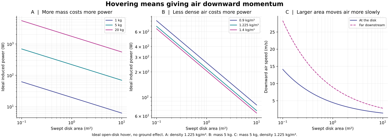
Run generate.py with Python, NumPy and Matplotlib. Independent momentum and kinetic-energy reconstructions check all cases; scaling checks cover mass, area and density. Passing these checks verifies the calculation's consistency, not a flight claim.
06 / USE THE MODEL TO ASK BETTER QUESTIONS
For a proposed hovering device, record total mass, swept area, thrust and power at the same operating point. A larger area may reduce ideal power while adding mass, size and control constraints. This page does not select a safe aircraft design.
Identify power connections, expelled matter, supports and external fields. Include return leads and reaction forces.
A proposed force study would record calibrated force, current, field map and uncertainty, including zero and reversed-current controls. No such measurements are reported here.
Explain discrepancies before claiming a new mechanism. A local component force or a field-energy estimate cannot replace measured net force and energy accounting.
READ FURTHER
NASA Glenn · Propeller analysis explains momentum flow and ideal disk velocity.
NASA Glenn · Thrust force includes momentum and pressure terms.
OpenStax · Force on a current-carrying conductor explains forces and complete-loop cancellation in a uniform field.
NASA · Ion propulsion describes conventional propellant acceleration and neutralization.
MIT · Experiments in electroaerodynamic propulsion is primary research on atmospheric ionic-wind propulsion; fixed-wing flight is distinct from hovering.
Revised 28 September 2026. Conventional teaching models with explicit system boundaries; no new engine or measured performance is claimed.
Xenon gas can be ionized: NASA's Deep Space1 engine used electrons to remove electrons from xenon atoms. That established process contradicts a blanket claim that free xenon cannot be ionized; it does not validate a different proposed chemical activator. NASA/JPL's original engine report
A system that first liquefies air and later expands and heats it also needs an account of the cooling and compression work, heat transfers and any consumed materials. Downward exhaust identifies a reaction partner, but does not determine the full system's efficiency or required input power. The ideal rotor example above does not model that cycle.
THE PROPOSALS / KEEP THE MISSING PIECES VISIBLE
One proposed air-breathing cycle would cool air, heat it and direct the exhaust downward. The available concept sketch has no scale, measured flow, vehicle mass, measured thrust or complete energy balance. Two component labels may be reversed, so the sequence is uncertain. The ideal rotor exercise is a conventional hover-power comparison; it does not test this cycle. Diagram method and limits · JSON
Simple version: A magnetic-field reading is not a push. To show that a vehicle moves, measure the force on the whole vehicle and identify what pushes back.
For a scale check, consider an illustrative field value of 0.46 T at 10 m. No calibrated field measurement, vector map, current geometry, duration or force measurement is supplied here, so this value is an assumed input, not experimental evidence.
This is an illustrative calculation, not a reconstruction: for a chosen ideal circular loop with radius a = 6.59 m and axial distance z = 10 m, B = μ₀NIa²/[2(a²+z²)3/2] gives about 28.96 million ampere-turns for the assumed 0.46 T field. Here N is the chosen turn count and I the current; neither is specified. The same ideal loop gives a central field of about 2.76 T. Resistance, coil mass, cooling, power and measurement uncertainty are omitted, so the calculation cannot establish feasibility.
At 0.46 T, the vacuum field-energy density is about 84.2 kJ/m³. That is a local energy per volume, not total stored energy, usable power or force. Propulsion still requires a complete momentum and energy balance with the field source or another reaction partner. Download the standard-library Python reproduction script and its machine-readable inputs and results. The script reproduces only the selected ideal-loop scale check; it is not a vehicle model.
A separate proposal invokes particle orientation and a changed reference framework, without usable dynamics or complete balances. A shape can still be studied: compare two ways of bounding its volume. That calculation does not show a machine travelling through it. For an established force-law comparison, inspect the complete-circuit model below.
Travel-time claims need defined distances, clock conventions and observations. They remain unverified in the idea register. Navigation, artificial gravity and voice control are supporting topics; successful sensing or an accepted command does not supply thrust.
The diagram is a simplified teaching illustration of possible components in an air-processing cycle. It does not establish their order, internal mechanism or operation. No measured flow, power, thrust or complete energy balance is provided.