Imagine this
Heat moves from hotter things to cooler things. A blanket can slow how fast warmth leaves, but it cannot make heat disappear. Follow heat through every layer and part of the journey.
THE FIELD GUIDE / 005 · ENERGY & HEAT
A warm mug, a thick coat, and air rushing past. All show how heat moves or changes form.
Heat travels from warmer things to cooler ones. A layer can slow that journey. When fast air slows, some motion energy can warm the gas. Start with the simple version, then explore the models.
Start with the simple version ↓Heat moves from hotter things to cooler things. A blanket can slow how fast warmth leaves, but it cannot make heat disappear. Follow heat through every layer and part of the journey.
Today, heat-flow models help compare insulation, cooling time and heating needs in a stated situation. A future cooling design would still need a full-system test.
The calculations use things we chose to assume. Real airflow, how parts touch, material properties and changing conditions still need checking.
Read-aloud starter; not yet tested with children. The fuller science, data, figures and sources follow below.
THE SIMPLE VERSION · NO BACKGROUND NEEDED
Think of a warm mug in a cool room. Heat leaves the mug and warms the air and your hands. A thick layer around an object can slow that journey, a little like a warm coat slows how quickly your body loses heat.
A coat does not make heat disappear. If the surroundings stay warm long enough, the object inside will warm too. And when warm air slows down, some of its motion energy can become energy inside the gas, so the gas gets hotter.
For a liquid moving through a warm pipe, each small bit of liquid spends less time beside the warm wall when it moves faster. It may warm less on its way through, even though more liquid passes each second.
Knowing where heat goes helps engineers design building insulation and temperature control for spacecraft instruments. That can support comfort, lower heating and cooling demand, and protect equipment when the real design is measured and tested. U.S. Department of Energy: home insulation · NASA: spacecraft temperature control
The curves below are simplified calculations, not measurements of a real material or vehicle. They do not show that food is safe, that germs have been killed, or that medicine stays within a safe temperature range. Those questions need their own evidence and tests; see the separate food and hygiene chapter.
Next, follow the rigorous layer: gas slowing, heat crossing layers, liquid flow and their assumptions, graphs and downloadable methods. The simple explanation and the scientific account use the same evidence.
01 / MOTION BECOMES INTERNAL ENERGY
Imagine bringing a stream of air to rest without exchanging heat with its surroundings. The final gas temperature is called its stagnation temperature. Mach number measures speed relative to the local speed of sound.
Temperatures use kelvin (K), an absolute scale. Subtract 273.15 to convert K to °C.
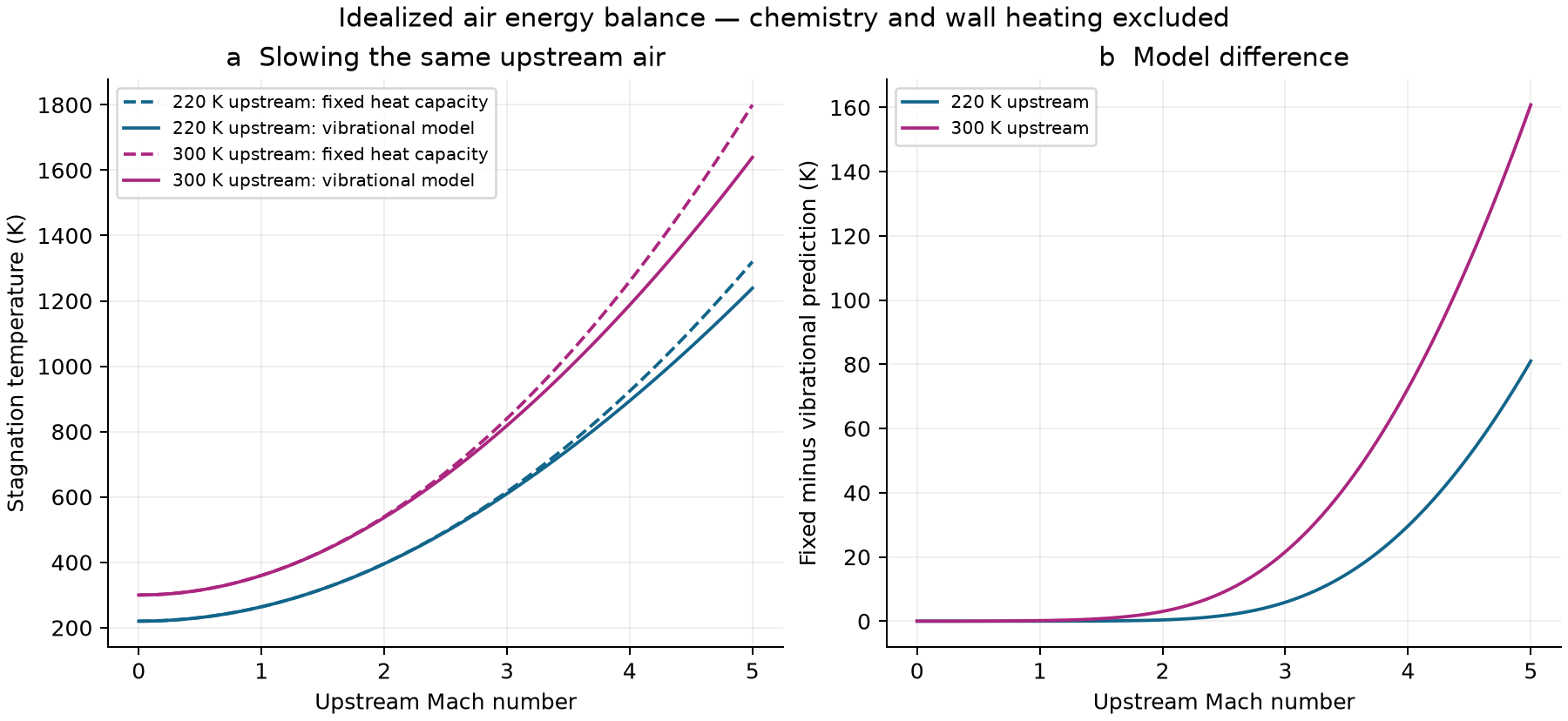
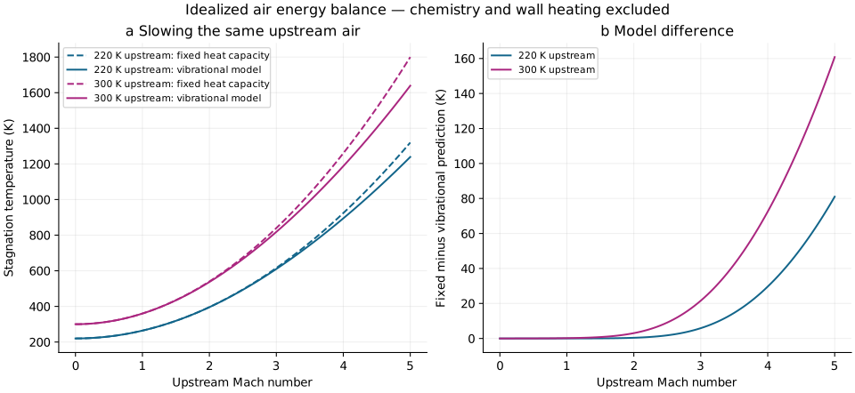
Dashed pink: fixed heat capacity. Solid blue: molecular vibration included. The dot marks your selected speed. At high temperatures both models omit chemical changes in the gas.
This is gas temperature, not wall temperature or heat flux. A real surface also involves flow geometry, heat transfer, radiation and the material response.
02 / WHY THE CURVES SEPARATE
At lower temperatures, a simple model assigns nearly constant heat capacity to air. At higher temperatures, more energy can enter molecular vibration. The same energy input then produces a smaller temperature rise.
Mach number alone is insufficient. Change the incoming temperature and the final temperature changes too.
The blue curve includes one additional physical effect. It is not a complete real-air calculation: dissociation, ionization and chemical nonequilibrium are absent.
03 / FOLLOW THE TRANSFER
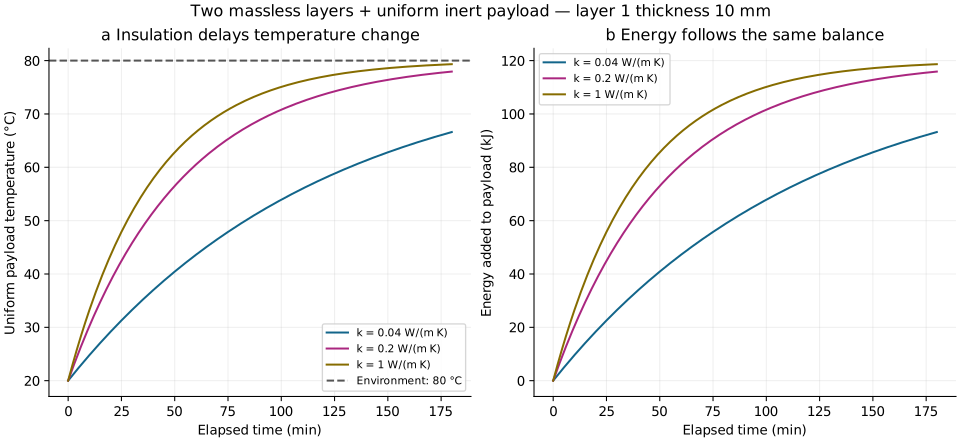
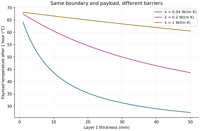
An inert, well-mixed payload starts at 20 °C. Its surroundings stay at 80 °C. Heat crosses an external convection boundary and two ideal layers. Increase the first layer’s thickness and see how slowly the payload warms.
Higher conductivity lets heat through more easily. These are illustrative values, not certified material specifications.
Insulation delays change; it does not create cold. Given enough time, this payload approaches 80 °C for every finite resistance.
Area A = 0.1 m²; payload heat capacity C = 2,000 J/K; external convection h = 10 W/(m² K); second layer thickness = 2 mm and conductivity = 0.2 W/(m K). Both layers have negligible heat storage and perfect contact. Heat travels in one dimension.
Resistance R = 1/(hA) + L₁/(k₁A) + L₂/(k₂A), in K/W. The energy balance C dT/dt = (Tᵦ − T)/R gives T(t) = Tᵦ + (T₀ − Tᵦ) exp[−t/(RC)]. Heat rate is (Tᵦ − T)/R; energy gained is C(T − T₀). The layer-interface temperature follows the same instantaneous heat rate through both layers.
This quasi-steady layer model cannot show a heat front propagating through a massive shield, melting, ablation, radiation, stress or structural failure.
04 / LIQUID IN MOTION
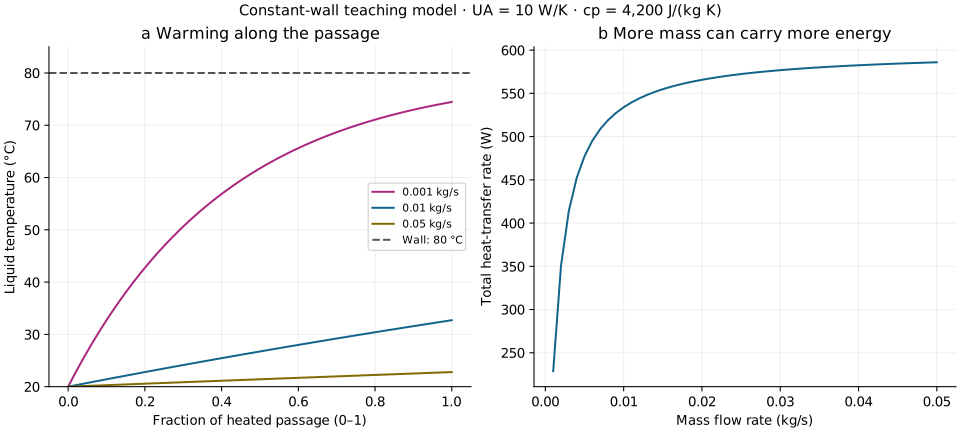
A liquid enters a heated passage at 20 °C. The wall stays at 80 °C. Speed up the flow: each kilogram receives less energy during its passage.
For fixed overall conductance UA = 10 W/K and specific heat cₚ = 4,200 J/(kg K), the steady plug-flow energy balance gives Tₒᵤₜ = Tᵦ + (Tᵢₙ − Tᵦ) exp[−UA/(ṁcₚ)]. This separate passage model assumes constant properties, no phase change and negligible axial conduction.
UA describes the whole passage; it is not taken from the flat layers above. It is deliberately held fixed as flow changes; a real passage’s conductance may also change with flow. Pressure drop, flow mixing, heater control, cleaning and food safety require separate analysis.
05 / LOOK INSIDE
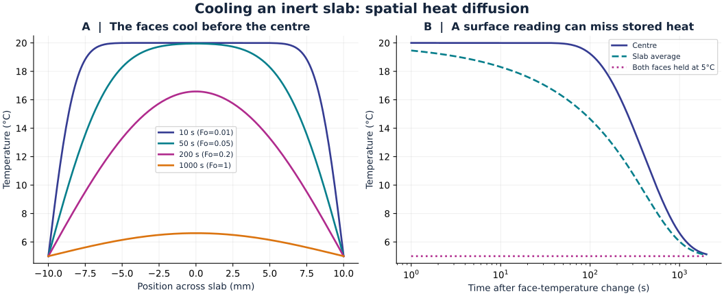
Now consider a different object: a solid sheet 20 mm thick, initially at 20 °C. At time zero, both faces are held at 5 °C. Heat inside must diffuse toward the faces. Move time forward to see the interior catch up.
The illustrative thermal diffusivity is 10⁻⁷ m²/s. Larger diffusivity means a temperature disturbance spreads faster.
A surface sensor alone can miss heat still stored inside. In this model, doubling the sheet thickness makes the same temperature profile take four times as long: the diffusion timescale is proportional to thickness squared.
This calculation resolves temperature across an inert solid. It assumes a wide plane sheet, constant properties and perfectly controlled face temperatures. It does not use the earlier convection-and-layer boundary conditions, so these are separate examples, not competing predictions of the same object.
The heat equation is ∂T/∂t = α ∂²T/∂x². Here the half-thickness L is 0.01 m, and the Fourier number Fo = αt/L² measures elapsed time relative to diffusion. A 64-term cosine series solves the stated fixed-face problem; the downloadable code gives its coefficients.
The face temperature changes instantaneously in this idealization. The earliest displayed time is one second; we do not calculate the instantaneous boundary jump. There is no freezing, internal heating, edge loss, fluid movement or temperature-dependent material behavior.
A uniform-temperature approximation is useful only when internal gradients are small. For convection at an object’s surface, the Biot number Bi = hL꜀/k helps assess that condition; L꜀ is volume / surface area, and k is the object’s conductivity. Bi around 0.1 is a common heuristic, not a universal switch. The fixed-face example here deliberately permits substantial gradients.
These are inert-material calculations. They do not establish biological preservation, food safety or human heat-exposure limits.
INSPECT YOUR SETTINGS
These tables follow your current controls. Downloads include the more finely sampled curves, units and selected inputs.
| Mach | Fixed capacity (K) | Vibrational (K) |
|---|
| Time (min) | Payload (°C) | Heat rate (W) | Energy gained (kJ) |
|---|
| Passage fraction | Temperature (°C) | Heat received so far (W) |
|---|
| Position from left face (mm) | Temperature (°C) |
|---|
A HISTORICAL OBSERVATION · LIMITED EVIDENCE
A 1935 Nature account describes one firewalking demonstration. The observer recorded a sole-surface temperature of about 93.2 °F (34.0 °C) around 20 minutes before the walk and about 93.0 °F (33.9 °C) roughly 10 seconds afterward. The account says the feet had been washed and dried about 15 minutes earlier. These are observations from one reported event, not a controlled test of why it happened.
| Observation | What it can support | What it cannot establish |
|---|---|---|
| Two sole-surface readings, before and shortly after one event | A limited record of that reported demonstration | The cause, heat flux during contact, or a sweat-and-evaporation effect |
| No controlled dry-versus-wet comparison or detailed ember measurements | A reason to keep the explanation open | A general safety claim or a repeatable protection method |
The models on this page use specified, inert boundaries. They do not model skin or reproduce firewalking, and this site does not recommend trying it. Read the 1935 Nature report.
06 / REPRODUCIBLE CALCULATIONS
DETERMINISTIC TEACHING MODELS · NO EXPERIMENTAL MEASUREMENTS
Run each downloaded Python script in its own folder with Matplotlib installed; the spatial study also requires NumPy. The scripts write beside themselves. File headers identify units and prescribed inputs.
An independent finite-difference solution approaches the sheet’s series solution as its grid is refined: maximum differences at four tested times fall from 0.03037 to 0.007668 to 0.001921 °C with 100, 200 and 400 intervals. This checks the specified calculation, not a real material. For the liquid, a separate numerical integration over 100 segments differs from the analytical outlet formula by less than 0.000001 °C across the exported flow range.
At Mach 0, both gas models return the incoming temperature. With air at 220 K and Mach 2, the fixed-capacity result is 396 K. Initially, the payload is 20 °C with zero energy gained. After one time constant RC, it has covered 63.2% of the temperature difference, reaching 57.9 °C.
The fixed-capacity gas relation is Tₜ = T[1 + (γ − 1)M²/2], with γ = 1.4. The vibrational relation and characteristic temperature 5,500 °R (3,055.56 K) follow NASA’s model below; the implicit equation is solved by bisection.
FROM A MODEL TO A TEST
Suppose an inert instrument package must stay below 40 °C for one hour in the model’s 80 °C surroundings. It starts at 20 °C and has the same 2,000 J/K heat capacity. Solving the temperature equation requires total resistance of at least 4.44 K/W.
With the other settings unchanged and first-layer conductivity 0.04 W/(m K), the ideal calculation needs about 13.4 mm of that layer. At 14 mm, the predicted temperature after one hour is 39.4 °C. If conductivity is 20% higher than assumed, the same 14 mm layer predicts 41.7 °C after one hour and misses the requirement. This sensitivity is illustrative, not a measured uncertainty distribution. This is a calculation for a hypothetical requirement, not a material recommendation or a certified enclosure.
These are proposed measurements, not results supplied by this page. Sensor lag, uncertain conductivity, imperfect contact and edge losses can all shift the curve. A close numerical solution cannot remove those physical uncertainties.
07 / WHAT THIS COULD IMPROVE
Estimate how resistance and heat capacity change temperature drift before selecting materials for controlled measurements.
Understand why a faster flow can leave a passage cooler even when its wall temperature stays the same.
First estimate the flow state, then heat transfer, then the object’s response. No single gas-temperature number answers all three.
READ FURTHER
NASA Glenn · Stagnation temperature and real-gas effects supplies the gas relations.
MIT · Thermal resistance circuits derives transfer through layers.
MIT · Dimensionless analysis explains the uniform-temperature approximation.
MIT · Heat exchangers, uniform wall temperature derives the exponential liquid-temperature relation.
MIT OpenCourseWare · Transient heat conduction gives the fixed-face plate solution used for the sheet.
Revised 27 September 2026. Original educational calculations, not a peer-reviewed material or flight evaluation.
One proposed membrane is assigned a temperature of 0.000825 kelvin—0.825 millikelvin above absolute zero. The description provides no cooling power, heat-leak budget, material behavior or temperature measurement supporting that condition. The ordinary-temperature examples here cannot be extrapolated to demonstrate it.