Imagine this
A straw looks bent where it goes into water. Light can bend too when it travels through places that change it. This page asks if changing a material could guide light; it does not show a finished lens.
THE FIELD GUIDE / 019 · OPTICS
Air can bend light when its properties change from one place to another. The shimmering view above a hot road is a familiar sign: changing air bends different light paths by different amounts.
This chapter separates three questions: can a gradient bend light, can heat create that gradient, and can a device hold it steady enough to form a useful image?
A straw looks bent where it goes into water. Light can bend too when it travels through places that change it. This page asks if changing a material could guide light; it does not show a finished lens.
Today, optical methods can make heat flow visible in experiments. Controlled gas optics is a possible next step, not a demonstrated instrument.
The page calculates small refractive-index changes and separates heating from ray bending. A working gas lens and its stability have not been shown.
Read-aloud starter; not yet tested with children. The fuller science, data, figures and sources follow below.
Refractive index describes how slowly light travels through a material compared with vacuum. If the index changes across a beam, its path gradually curves toward the higher-index region. You do not need a sharp glass surface for refraction.
At fixed pressure and composition, warmer gas is usually less dense and has an index closer to one. A temperature difference can therefore create an optical gradient. Moving air, pressure changes and uneven heating also change that gradient.
A constant sideways gradient steers a beam. Focusing several rays to one place needs a suitable spatial profile. The simple steering experiment below is not a focusing lens or an image-quality prediction.
TRY THE MODEL
Our hypothetical index changes linearly across the ray: n(y) = n₀ + gy, with n₀ = 1.00027. The ray starts horizontally at y = 0. Positive y points upward.
Vertical displacement is magnified. Read the numerical output for the physical scale. Doubling the distance multiplies displacement by four in this particular model.
Turning on a heater does not specify the resulting optical shape. Energy must first be absorbed, then move through the gas and its container. Gas motion can carry heat away. Sensors and feedback must detect and correct departures from the desired profile.
In particular, an electromagnetic heater needs a measured coupling mechanism: its frequency, absorbed power and the gas response matter. A count of heating elements alone cannot establish a useful temperature field.
The chain to test: electrical input → absorbed heat → temperature and density field → refractive-index field → ray paths → image quality. This chapter calculates only selected links. It does not simulate absorption, convection, heater control or the resulting image.
For a separate, illustrative fixed-pressure gas approximation, n − 1 is proportional to 1/T. We assign n = 1.00027 at 293 K; this is not a calibrated material specification.
Uniform heating changes this index value but does not create a sideways gradient by itself. This temperature control is deliberately separate from the ray experiment; it is not a calculation of the heater needed to produce its gradient.
Schlieren and related optical methods make refractive-index variations visible. They help study hot air, gas flow and thermal plumes. Here the changing light path is a measurement signal, rather than a stable lens.
A research study could ask whether a measured temperature profile can steer or focus a beam reproducibly. It would need to compare stability, aberrations, aperture and energy demand against ordinary optical components before claiming a practical advantage.
REPRODUCIBLE NUMERICAL STUDY
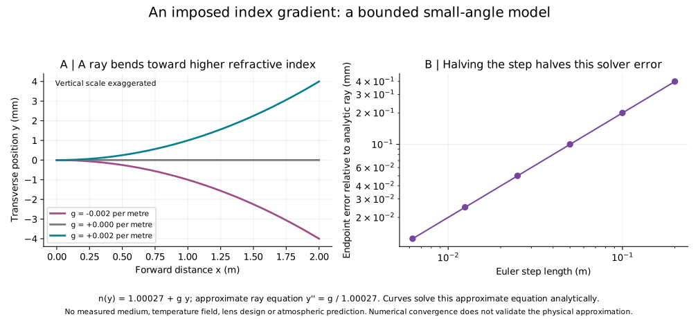
603 ray samples, 61 separate temperature-index values and 6 convergence cases are supplied. Reversing the gradient reverses the bend; the zero-gradient ray remains straight.
For small slopes and small index variations, d²y/dx² ≈ g/n₀. Its solution is y = y₀ + s₀x + gx²/(2n₀), where s₀ is the initial slope. The displayed angle uses the small-angle approximation angle ≈ slope, in radians.
Our largest displayed slope is about 0.004, so the small-angle condition is satisfied. The calculation assumes a static prescribed gradient. It omits diffraction, boundaries, absorption, fluctuations and any thermal or fluid evolution. Agreement with an analytical solution checks the calculation, not the existence or quality of a physical device.
Measure the actual index or temperature field; state pressure, composition and wavelength; compare predicted and measured ray displacement; then measure focal behaviour, distortion and stability over time. The result must remain reproducible when conditions change.