Imagine this
Two thermometers can both be wrong in the same way. We can compare them, but joining their answers will not always fix a mistake they share. They may also take their readings at different times.
THE FIELD GUIDE / 025 · SENSORS AND ESTIMATION
More sensors can help us understand the world. But agreement is useful only when we know what was measured, when it was measured and which errors the sensors share.
Two thermometers can both be wrong in the same way. We can compare them, but joining their answers will not always fix a mistake they share. They may also take their readings at different times.
Fusion methods help separate random spread, shared bias and timing errors. A real sensor system needs calibration and ground-truth checks.
The page uses analytical and synthetic examples; it does not certify a particular sensor package.
Read-aloud starter; not yet tested with children. The fuller science, data, figures and sources follow below.
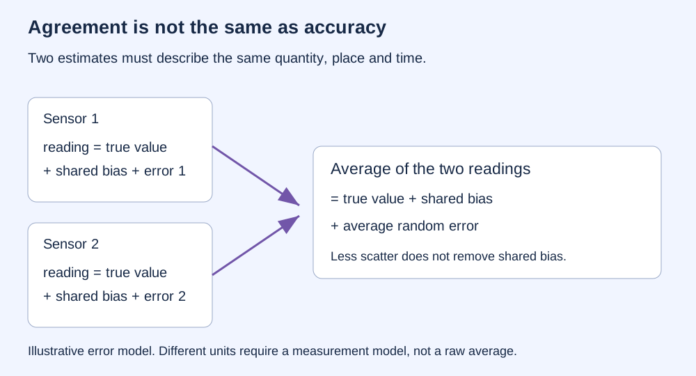
Imagine two thermometers calibrated against the same faulty reference. Both read too high. Their average may fluctuate less, yet it remains too high. Random errors that vary independently can partly cancel; a shared offset survives averaging.
A camera and a vibration sensor can offer different clues about a machine. Their raw readings have different units and cannot simply be averaged. We first need a model that connects each reading to the question we want to answer. NIST: correlation in measurement uncertainty
SAME QUANTITY, EQUAL NOISE
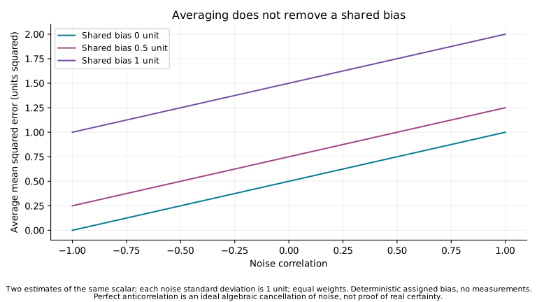
Each invented sensor measures the same constant quantity. Each has random error with standard deviation 1 unit. Correlation describes how strongly their random errors move together: −1 means exact opposition, 0 means no linear correlation, and +1 means identical random errors in this equal-noise model.
Root mean square error includes both the assigned random variation and the fixed offset. The spread alone leaves out that offset. Try correlation +1: averaging brings no reduction. Try −1: random errors cancel exactly in this mathematical limit, but a shared offset still remains.
No instrument has been tested here. Correlation and offsets are assigned, not estimated. Zero correlation does not generally imply independence; it produces the same variance calculation for this average.
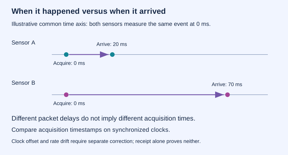
A robot travelling at 2 metres per second moves 20 centimetres in 100 milliseconds. Two accurate position sensors can therefore disagree by 20 centimetres if they observe it 100 milliseconds apart.
The timestamp should describe when a reading was acquired. When its packet arrives is a different event. A clock can start ahead or behind, run slightly faster, and share a network whose delays change from packet to packet. NIST: synchronising distributed measurement clocks
| What happens | What to check |
|---|---|
| Clock offset | Do the clocks agree at the same physical instant? |
| Clock drift | Does their disagreement grow with elapsed time? |
| Network delay and jitter | How late and how variably do packets arrive? |
| Missing or late packets | Which expected sequence numbers arrived, and which arrived before the deadline? |
A wearable network can receive nearly every packet and still have poorly aligned readings. Duplicate packets must not inflate the delivery fraction. Buffering may help align arrivals but adds waiting time; interpolation estimates gaps rather than recovering missing measurements. More frequent transmission also uses bandwidth and energy. None of these timing checks establishes medical accuracy or a miniature device design.
CONSTANT SPEED AND CLOCK RATE
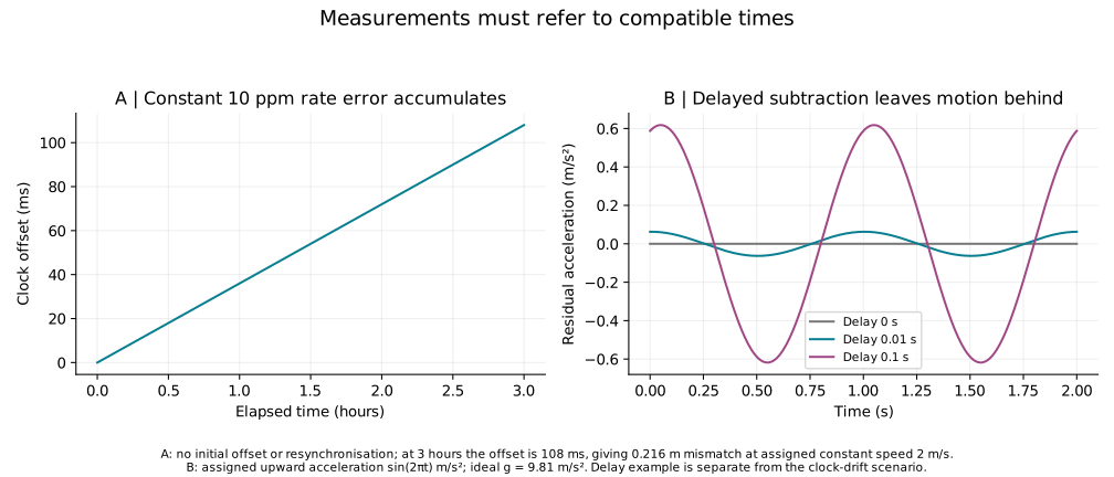
These are two separate calculations. The position result uses the acquisition offset slider, not the accumulated clock offset. A constant relative rate error of 10 parts per million produces 108 milliseconds over three hours if it is never corrected. Synchronisation can change that outcome.
In our simple upward-axis convention, gravity points down and has magnitude g = 9.81 m/s². An ideal accelerometer measures specific force f = a + g along this axis. A supported stationary sensor reads +g. In ideal free fall, a = −g and its reading is zero.
To infer gravity on a moving platform, we need an additional estimate of the platform's acceleration: ĝ = f − a. Accelerometer measurement principles. Tilt changes which part of the force lies along each sensor axis. Bias, vibration and an incorrectly timed correction can all leave a misleading residual. Gravity alone also does not uniquely identify altitude without a field model and reference.
IDEAL UPWARD AXIS · SYNTHETIC MOTION
The platform's acceleration is a(t) = sin(2πt) m/s², repeating once per second. We subtract an otherwise exact acceleration estimate delayed by Δt. The remaining error is a(t) − a(t − Δt).
Exact maximum absolute residual for this continuing sinusoid: . Zero delay cancels motion exactly in this ideal model. This is not a working gravimeter: rotation, gradients, sensor noise, vibration and calibration error are omitted.
A CHOSEN GEOMETRIC RULE · NOT A TRAINED MODEL
Two familiar categories are represented by centres A and B. Our invented rule assigns the nearest label only when the point lies within the chosen radius. An equal-distance tie withholds the label. Coordinates are dimensionless features, not real sensor measurements.
This hand-picked point is declared unfamiliar, yet the rule accepts A. Its hidden category is assigned for illustration, not learned.
Circles show a chosen acceptance rule, not probabilities. Shrinking them makes the rule answer less often. It cannot guarantee that every unfamiliar case is rejected: an unfamiliar point may sit close to a familiar centre. A rejected familiar point is also possible. Missing input is a separate problem, not another point on this map.
A real evaluation must report accepted-correct, accepted-wrong and rejected familiar examples, plus accepted and rejected unfamiliar examples with their own denominators. A small score is not automatically a calibrated probability. There is no training dataset, test population or accuracy percentage in this schematic. Primary research on recognising unfamiliar classes
Today: a robot combines camera and motion readings to estimate movement; a production line synchronises measurements made at different stations. Both need calibration and timing checks, and an independent way to assess whether the combined estimate is useful.
A future direction: monitoring systems could identify faulty inputs, admit unfamiliar cases and continue with the evidence they can trust. The benefit must be tested against a single-sensor baseline, including shared errors, drift and failures. More sensors alone are not proof of improvement.
These examples explain measurement principles. They do not establish a new gravity instrument, a clinical wearable or a classifier that recognises every unknown.
REPRODUCIBLE STUDY
| Assigned case | Calculated result |
|---|---|
| Correlation 0, no shared offset | Average variance 0.5 units²; random spread about 0.707 units |
| Correlation 1, no shared offset | Average variance 1 unit²: no gain from averaging |
| Correlation 0, shared offset 1 unit | Mean squared error 1.5 units² |
| 10 parts per million, 3 hours, no correction | 108 ms accumulated clock offset |
| 1 Hz, 1 m/s² motion, 10 ms delayed subtraction | Maximum residual about 0.06282 m/s² |
For equal random-error standard deviation σ = 1 and equal averaging weights, Var(mean) = σ²(1 + ρ)/2. With a shared deterministic bias b, MSE = Var(mean) + b². No Gaussian distribution is required for these moment identities. Correlation must lie between −1 and +1. Exact cancellation at −1 is an ideal limit.
Clock drift in seconds = rate error in parts per million × 10⁻⁶ × elapsed seconds. Constant-speed mismatch = speed × acquisition offset. Motion residual = sin(2πt) − sin(2π(t − Δt)); its maximum absolute value over a full cycle is 2|sin(πΔt)|.
The rejection map uses Euclidean distance to A = (−1, 0) and B = (1, 0). Radius boundaries are included. Equal distances within 10⁻¹² withhold the label after the radius check; this tolerance does not expand the acceptance disks. At radius zero, only exact centres are accepted.
All numerical studies are synthetic calculations. The offline figures and browser controls use the stated equations; neither constitutes an experiment on hardware. Downloaded data and methods specify the sampled ranges. Continuous curves between points illustrate these analytic relationships.