Imagine this
Water travels through a pipe and then through soil to reach plant roots. The soil may slow it down even when the pipe delivers water. We must measure both parts and count how much water is needed.
THE FIELD GUIDE / 039 · SOIL AND WATER
A buried porous pipe releases water through connected pores. The water must cross the pipe wall, then move through the surrounding soil. Some may remain near roots; some may evaporate or drain deeper. Each step needs a different question and measurement.
Explore pressure and flow ↓Water travels through a pipe and then through soil to reach plant roots. The soil may slow it down even when the pipe delivers water. We must measure both parts and count how much water is needed.
The page compares simple flow calculations with a published field test of porous clay pipes. A farm would need to assess its soil, crop, water and layout.
The field example does not tell every farm how much to water. Soil, plants, water and pipe layout differ from place to place.
Read-aloud starter; not yet tested with children. The fuller science, data, figures and sources follow below.
A SIMPLE START · NO BACKGROUND NEEDED
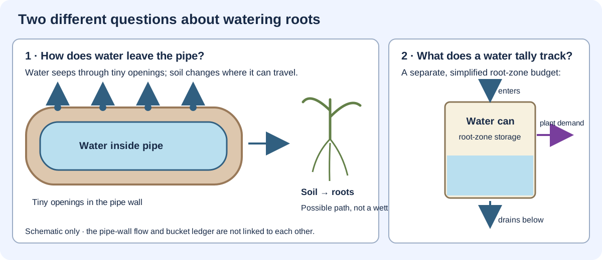
Imagine a tube under the soil with tiny openings in its wall. Water can seep out and move through the earth toward roots. Then ask a different question: how much water enters the root area, stays there, is counted as plant demand, or drains below?
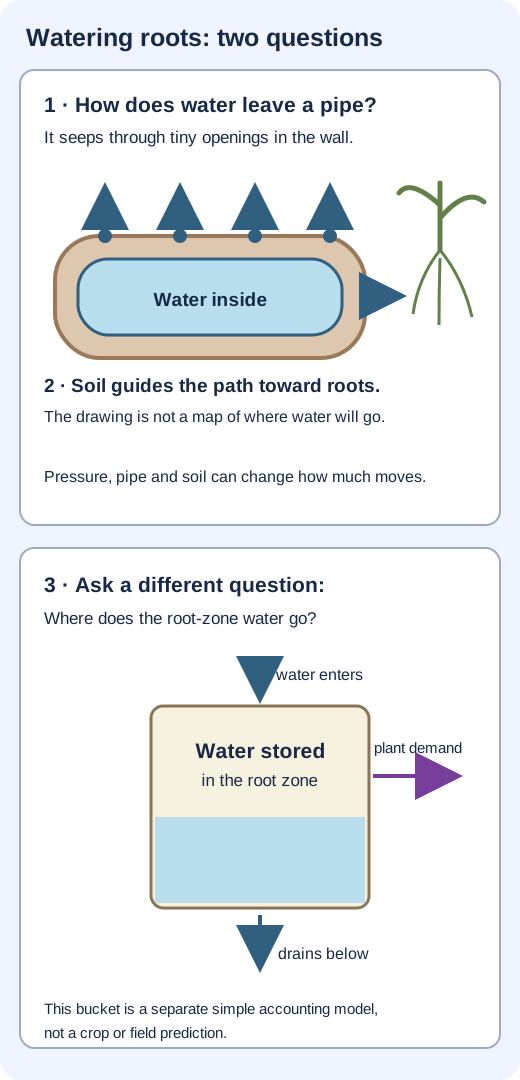
Tiny openings let water seep through the pipe wall. The material, wall and pressure can change how much moves.
Soil can guide water toward roots, sideways, or deeper. Different soil and weather can change the path.
A simple bucket model asks what enters a root-zone area, what stays, what is withdrawn to meet an assigned plant-water demand, and what drains away.
How could this help? Testing where irrigation water goes can help people compare ways of delivering water near crops. Real results depend on the pipe, soil, weather and plants. The models here do not show water saved or crops improved.
Scientists have tested porous clay pipes in a loam field and compared soil samples with computer estimates. See what that one field study measured ↓
Pressure inside a pipe helps drive water through its wall. The soil outside also resists flow, and that resistance changes as it wets and dries. The pipe is part of a coupled system, not a tap with a universally fixed delivery rate.
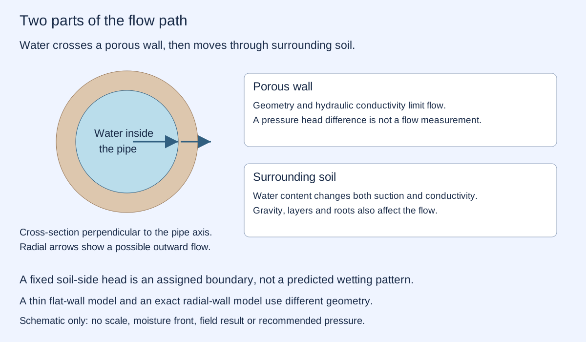
The material's hydraulic conductivity describes how readily water flows under an imposed head gradient. It is not the same as the fraction of empty pore space. Conductivity has units of length per time; intrinsic permeability has units of area.
SATURATED HOMOGENEOUS WALL · FIXED BOUNDARY HEADS
Imagine flattening a small, thin patch of the pipe wall. Keep its area at 0.10 m² and thickness at 5 mm. Change the hydraulic conductivity and the difference in water head across it. Positive head drives flow outward; reversing the head reverses the calculated flow.
A metre of water head represents energy per unit weight. With the same elevation on both sides, 1 m of pressure head corresponds to about 9.81 kPa for the assigned water density 1,000 kg/m³. A soil-side suction or a height difference also contributes to total hydraulic head; a pressure reading alone need not equal the total difference.
Darcy's law here is Q = KAΔH/L, with Q in m³/s, conductivity K in m/s, area A in m², thickness L in m and head difference ΔH in m. Multiplying Q by 3,600,000 gives litres per hour. The sign is defined as outward flow. This is a steady, saturated, uniform, thin planar wall with assigned boundary heads. Soil resistance, air entry, pipe curvature, clogging and pressure loss along the pipe are omitted.
A uniformly saturated cylindrical wall instead gives Q = 2πKℓΔH / ln(rₒ/rᵢ), where ℓ is pipe length and rᵢ/rₒ are the inner/outer radii. These geometries have different areas and must not be mixed. The interactive uses only the planar approximation.
USGS explains Darcy flow and hydraulic gradient. Hydraulic conductivity and dimensions here are invented teaching inputs. This is not a predicted flow for a particular pipe, a complete irrigation network or a recommended operating pressure.
Dry soil can exert stronger suction, yet its partly air-filled pathways may conduct water much less readily. The pressure difference and the ability to transmit water both matter. As water moves, those properties change.
Soil texture, gravity, retention, roots and spatial variations determine where the water goes. A realistic wetting map needs appropriate soil relationships and a model of unsaturated flow. The fixed outer head above is a declared boundary condition, not a simulation of changing soil moisture.
Siyal and Skaggs' 2009 porous-pipe study measured wetting in a loam field and compared it with a flow model. It examined four pressure heads over five days. Those results concern the tested conditions; they do not establish a universal water saving or validate the unspecified project proposal.
Salt accumulation, clogging, root intrusion, variable pipe material, pressure loss and maintenance can alter practical performance. A wall calculation does not remove these questions.
30-DAY ACCOUNTING EXAMPLE · NO CROP MODEL
Now consider a separate root-zone storage ledger. It starts with 20 mm of available water above an arbitrary lower reference and has an assigned capacity of 40 mm. Each day, infiltrated irrigation arrives first; excess drains; then up to 5 mm is withdrawn to meet an assigned evaporation/transpiration demand.
One millimetre of water over one square metre is one litre. These depth units describe volume per area, not the physical depth of a wet soil layer. Infiltrated irrigation is already inside this budget; applied water that runs off or never reaches it is outside the stated input.
For each day: available = previous storage + irrigation; drainage = max(available − capacity, 0); actual withdrawal = min(demand, available − drainage); new storage = available − drainage − actual withdrawal. Unmet demand is demand minus actual withdrawal. Initial storage + cumulative input equals final storage + cumulative drainage + cumulative actual withdrawal.
Rainfall, capillary rise, runoff and lateral exchange are assigned zero here. The hard capacity and immediate drainage are accounting rules, not a model of real drainage at field capacity. There is no within-day timing, root distribution, soil retention curve, stress response or crop-yield prediction. The line joins daily end states; it does not resolve changes within a day.
The wall-flow model and this ledger are independent. Converting a pipe flow into field-scale infiltrated irrigation would require area, duration, distribution and losses. The site does not silently connect their outputs.
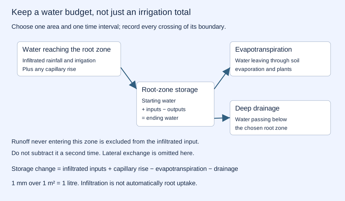
FAO's root-zone water-balance framework distinguishes available water, depletion, stress and drainage. Plant-available capacity depends on rooting depth and the difference between water contents at field capacity and wilting point. The arbitrary capacity above is not an estimate for your soil or crop.
Current use: porous irrigation can deliver water below the surface. Studying its transport helps compare designs and understand how soil conditions change delivery. Less surface exposure may reduce some evaporation, but that does not guarantee less total water use or better crop growth.
What a convincing improvement would show: compare similar crops, weather, soils, starting moisture and water quality. Measure water applied, changes in storage, drainage and crop outcomes over an appropriate period. Separate a reduction in supplied water from a change in yield or a transfer of losses elsewhere.
Future development: characterize wall material and clogging, measure how delivery varies along the network, then combine soil observations with bounded control. The source proposal supplies no usable dimensions, conductivity, maintenance data or field comparison. No prototype result is claimed here.
PUBLISHED FIELD STUDY + REPRODUCIBLE IDEALIZATIONS
Which design does this evidence support? The concept considered here proposes porous mortar, with pressure chosen for the soil and plant species. The published study below instead tests baked-clay pipes. Our interactive examples use assigned pressure head and a fixed daily water demand: they do not calculate a soil- or crop-specific pressure schedule, or demonstrate the proposed mortar design.
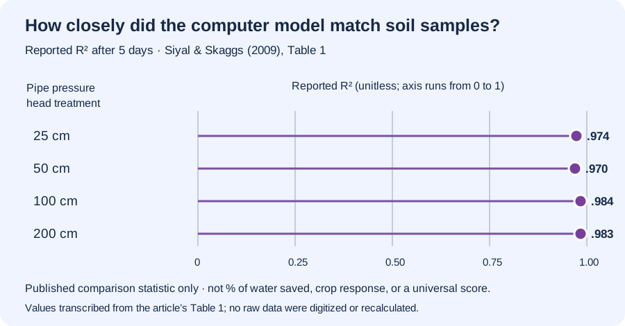
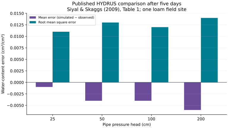
Siyal and Skaggs studied baked-clay pipes in loam soil at one field site in Pakistan. They measured soil-water content after five days at four pipe pressure-head treatments, then compared those measurements with HYDRUS computer estimates. Their Table 1 reports R² values of 0.970–0.984 for the tested cases. R² summarizes model-to-measurement agreement; it is not a percentage of water saved, crop growth, or a universal result.
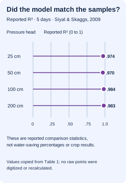
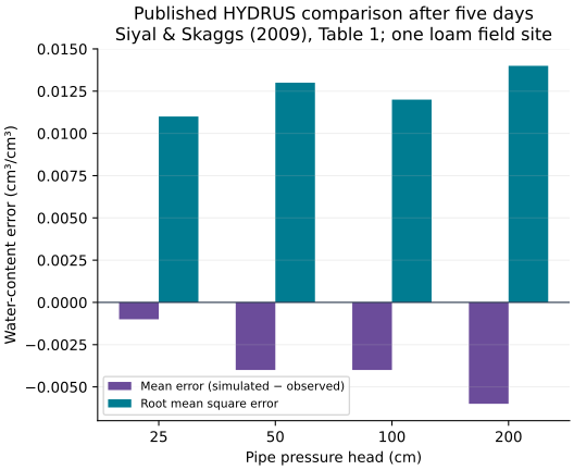
| Pipe pressure head (cm) | Mean error (cm³/cm³) | RMSE (cm³/cm³) | Reported R² |
|---|---|---|---|
| 25 | −0.001 | 0.011 | 0.974 |
| 50 | −0.004 | 0.013 | 0.970 |
| 100 | −0.004 | 0.012 | 0.984 |
| 200 | −0.006 | 0.014 | 0.983 |
The article distinguishes measured soil samples from simulated estimates. Its contour maps use kriging interpolation. We do not redraw those maps as if every location were directly measured, and we do not treat this one study as evidence of water savings or crop yield.
Now inspect the site’s separate idealized calculations. Their assigned parameters are not the study’s measurements and are not calibrated to this field experiment.
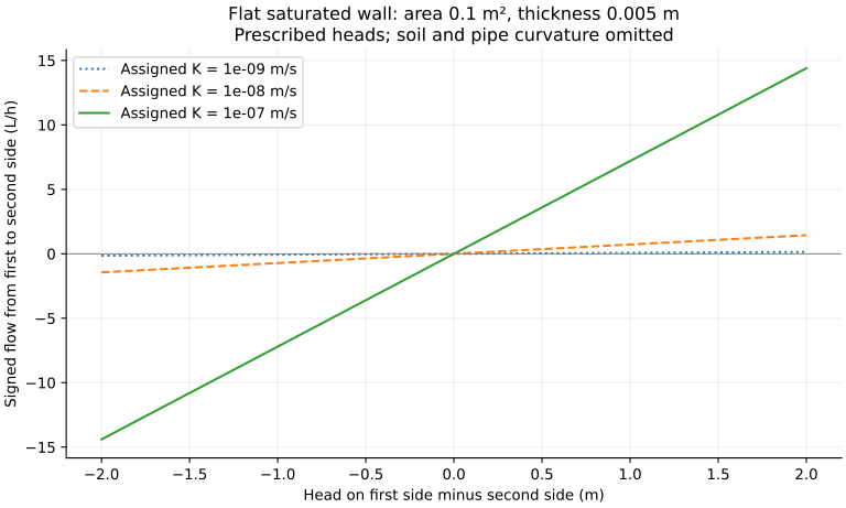
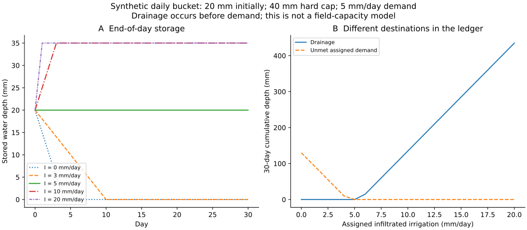
1,254 calculation rows: 603 wall-flow cases, 630 daily ledger states and 21 ledger summaries. The downloadable irrigation sweep steps by 1 mm/day; the interactive steps by 0.5 mm/day under the same rules.
Wall flow CSV · Daily ledger CSV · Ledger summaries CSV · Standalone reproduction script · Methods and limits · Runtime and parameters · Execution checks
Run with Python, NumPy and Matplotlib. The study checks flow direction, zero head, units, conservation on every day and over the full run, and the stated event order. Runtime and generator hash are recorded. No measured field data are generated by this script.
These calculations test equations and accounting rules under assigned assumptions. They are not field measurements, a crop recommendation or evidence of a particular percentage water saving.