Imagine this
Two people can write the same measured amount with different number symbols. Changing the symbols does not make the ruler more exact. We still have to check the measurement.
THE FIELD GUIDE / 031 · NUMBERS AND MEASUREMENT
A number can be written exactly while the measurement behind it remains uncertain. Changing its symbols, converting its units and checking the instrument are three different tasks.
Try a biased instrument ↓Two people can write the same measured amount with different number symbols. Changing the symbols does not make the ruler more exact. We still have to check the measurement.
Today, unit, base and uncertainty checks help people compare and reproduce scientific results. Careful reporting does not itself improve an instrument.
Exact conversion preserves a quantity; it does not reduce uncertainty, fix bias or correct a measuring device.
Read-aloud starter; not yet tested with children. The fuller science, data, figures and sources follow below.
Seventeen objects can be written as 17 in decimal, 15 in base twelve or 10001 in binary. Nothing about the collection changes. The base tells us what each position is worth: in base twelve, the places count ones, twelves, 144s and so on.
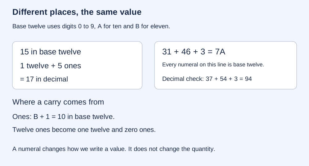
We use A for ten and B for eleven in base twelve. Adding one to B gives 10 in base twelve: write zero ones and carry one twelve. In the example 31 + 46 + 3 = 7A, all numerals are base twelve. The decimal check is 37 + 54 + 3 = 94. Unfamiliar symbols alone do not establish new mathematics; their rules must first be defined.
EXACT INTEGER ARITHMETIC
Change the value or its base. The table separates the written digit from its decimal value and the weight of its position. Powers mean repeated multiplication: 12² = 12 × 12 = 144.
| Digit symbol | Digit value | Place weight | Contribution |
|---|
Hexadecimal uses A through F for ten through fifteen. A different base changes the notation, not the quantity or the accuracy of a measurement. The previous chapter distinguishes this exact integer operation from rounding a continuous signal.
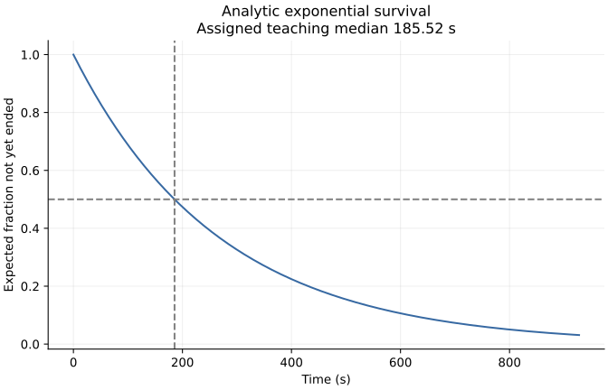
Imagine many independent objects, each leaving a group after a randomly chosen waiting time. In an exponential model, each has a one-half chance of remaining after one population half-life. A particular finite group fluctuates around the smooth population expectation.
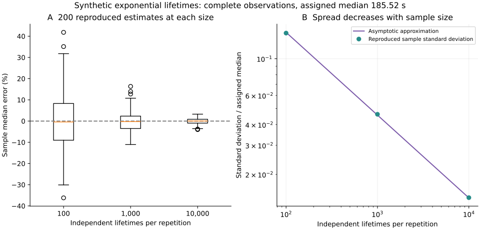
Generate a complete lifetime for every object, then put those lifetimes in order. The median separates the earlier half from the later half; for the even group sizes here, we average the two middle lifetimes. Repeating this process gives different median estimates. Larger groups tend to give a narrower spread.
The reproduced experiment uses 200 groups at each size: 100, 1,000 and 10,000 objects. Their median estimates have relative standard deviations of approximately 14.3%, 4.61% and 1.45%. These are simulated results, not measurements of radioactive material or a working clock. NIST describes the exponential lifetime model.
ANALYTIC EXPECTATION · NO NEW RANDOM RUN WHEN SLIDERS MOVE
The first control evaluates a large-sample approximation for the spread of estimated medians. It assumes independent, complete lifetimes. The second control shows the expected surviving fraction over time; it answers a different question.
Four times as many independent observations approximately halve the median's random spread. This is not an error bound or a confidence interval. Repetition does not remove a shared bias, missed events or a changing detector response.
At one half-life, the expected remaining fraction is 50%; at five it is 3.125%; at ten it would be 1/1,024. This refers to the surviving original population, not the total mass of original material plus products. An individual lifetime remains unpredictable in the model.
A population gradually disappears; it does not produce repeated cycles. The SI second is defined using a specified caesium atomic transition frequency, not spontaneous decay. Calling two processes atomic does not make their principles or precision equivalent. BIPM definition of the second.
One microcoulomb (µC), a unit of electric charge, equals 0.000001 coulomb (C). That factor is exact. If a reading is too high, expressing it in coulombs preserves the same physical error. Extra printed decimals do not repair it.
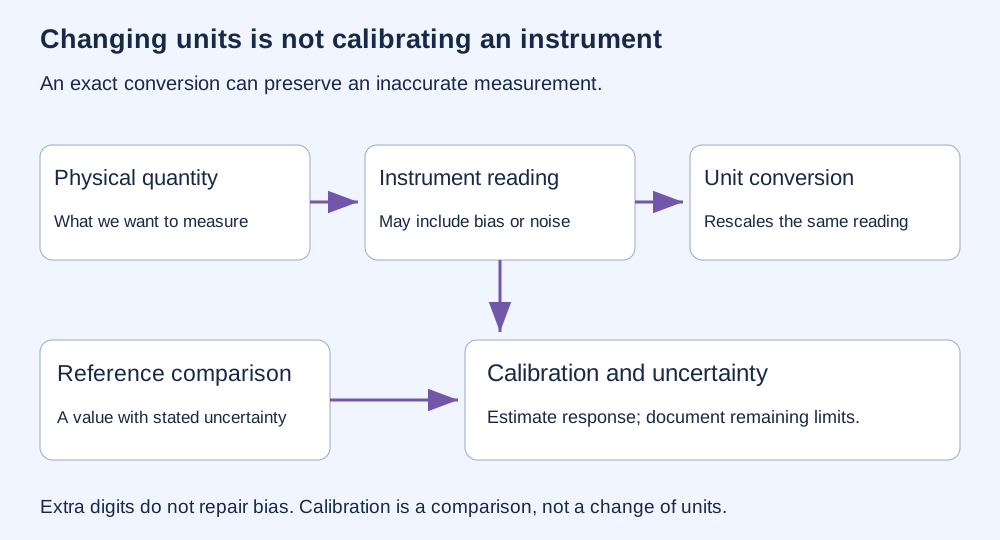
Calibration establishes a relationship between instrument indications and suitable reference values, with uncertainty. Applying a correction may use that relationship; adjusting the instrument changes the instrument itself. Calibration and adjustment are separate actions. NIST explains measurement traceability.
ASSIGNED INSTRUMENT RESPONSE · KNOWN COEFFICIENTS
We invent a true charge and an instrument response: reading = gain × true charge + offset. A gain of 1.05 exaggerates the signal by 5%; an offset adds the same amount to every reading. These coefficients are assigned exactly for teaching, not estimated from calibration data.
At the initial settings, a true 100 µC produces a reading of 107 µC. Converting it gives 0.000107 C; the 7 µC error remains. Subtracting the known offset and dividing by the known gain recovers the assigned 100 µC.
A real calibration would need reference measurements and uncertainties in the gain, offset and reference itself. This exact recovery is built into the hypothetical model; it is not evidence that real measurements can become uncertainty-free. Negative readings are allowed when an assigned negative offset outweighs the signal. Displayed values are rounded.
State the quantity, unit, method, reference and uncertainty. A documented chain of comparisons supports traceability; a number alone cannot supply it. An unfamiliar named unit without an operational definition has no demonstrated independent realization.
Taking the reciprocal of a duration gives a rate, but it does not establish that an event was detected or that a communication channel exists. Defining a length through a wavelength requires an identified reference and a measurement procedure.
A proposed length unit might be defined as a fixed number of wavelengths: L = Nλ. The multiplication is simple, but realizing the unit requires identifying the radiation, the conditions in which its wavelength is specified and the measurement method. Knowing only a proposed conversion into metres does not establish that the reference can be reproduced or how uncertain it is.
Today: software teams exchange numbers in different formats, laboratories compare readings, and engineers decide how many observations to collect. Explicit bases and units prevent interpretation mistakes; calibration records explain how a reading connects to a reference.
A useful next step: make data records carry the original indication, conversion rule, reference and uncertainty together. That could reduce reporting and comparison mistakes, provided systematic effects and real reference quality are assessed. It would not establish a new clock, unit or instrument accuracy.
Median: the middle of ordered observations; this study averages the two middle values for an even group.
Standard deviation: a measure of spread around the mean. Here it describes 200 estimated medians, not individual lifetimes; it is not an error bound.
Relative spread: here, that standard deviation divided by the assigned population half-life, expressed as a percentage.
Half-life: in this model, the time after which each original member has a one-half chance of still remaining.
Calibration: reference comparison to establish a measurement relationship and its uncertainty. Unit conversion changes how the same quantity is expressed.
REPRODUCED COMPUTATIONAL EXPERIMENT
| Complete lifetimes per group | 200-run relative spread | Large-sample approximation |
|---|---|---|
| 100 | 14.2794% | 14.4270% |
| 1,000 | 4.6149% | 4.5622% |
| 10,000 | 1.4471% | 1.4427% |
A single Python random-number stream, seed 21001, generates independent exponential lifetimes in group-size order 100, 1,000, 10,000, with 200 repetitions each. The assigned population median is 185.52 seconds, a teaching timescale with no isotope identity claim. Every lifetime is observed completely. The sample median averages the two central ordered values.
The 600 exported estimates come from an actual rerun, not reconstruction from three stored summary values. All numerical fields in those historical summaries were reproduced exactly on the recorded runtime. A standalone download can reproduce the experiment without the historical file, but cannot verify that historical comparison unless the file is present.
Population survival at time t is exp(−λt), with λ = ln(2)/T and assigned half-life T. The approximate relative standard deviation of the sample median is 1/[ln(2)√N]. It follows from the large-sample median variance 1/[4N f(T)²], where f(T) = λ/2 for this distribution.
The reported empirical spread uses the sample standard deviation of 200 median estimates (denominator 199), divided by the assigned T, not by their estimated mean. A finite-sample median need not be exactly unbiased. This formula is specific to this estimator and complete independent exponential observations; it is not a universal clock limit or a count-rate uncertainty formula.
The UI evaluates this approximation for group sizes from 100 to 1,000,000; the reproduced random experiment covers only the three tabulated sizes. Its fourfold comparison is analytic too. No fresh random samples are generated by moving a control.
Censoring, dead time, background signals, detector efficiency, shared errors and drift are omitted. Real uncertainty evaluation must include significant contributors and their relationships. NIST guidance on uncertainty propagation.
For the assigned instrument, r = ax + b, corrected x = (r − b)/a, and a reading in µC is multiplied by 10⁻⁶ to express it in C. The conversion factor is exact; the original reading and calibration coefficients in a real instrument are not thereby exact. These examples validate arithmetic and a declared simulation, not a new physical standard or clock.
MEASUREMENT / A FIELD READING IS NOT A NAME
The very simple version: A compass can notice a magnetic field. But it does not tell you the name of the thing making that field. A weaker magnet nearby and a stronger one farther away can sometimes give the same reading.
Understanding this helps us ask better questions about classroom magnets and environmental magnetic records. Measurements can reveal useful changes, but interpreting them needs information about location, direction, surroundings and the instrument. This lesson demonstrates a limitation of one reading; it does not say that additional measurements can never resolve an ambiguity.
Magnetic moment measures source strength in this model. It is not an object's mass, material label or measured sensitivity.
Constructed example: an ideal point dipole in free space, viewed on its axis. For a finite source, distance must be much larger than source dimensions. No finite magnet shape is specified or validated here.
Magnitude on the dipole axis, in nanotesla (nT). No background or instrument noise is included.
Try doubling the distance while keeping moment fixed: the contribution falls to one eighth. The model does not establish whether a particular sensor could detect it.
| Distance (m) | Axial contribution (nT) | Relative to 0.1 m |
|---|

On the axis of an ideal magnetic dipole, B=μ₀m/(2πr³), where m is magnetic moment in A m² and r is distance in metres. We use μ₀≈4π×10⁻⁷H/m, a classroom approximation rather than an exact modern-SI constant. With 1 T=10⁹ nT, B in nT is 200m/r³. Thus B(8m,2r)=B(m,r). This equality only concerns the one on-axis value being compared, not identical fields everywhere.
A real field measurement includes other contributions. Directional field components and total field magnitude are different quantities. General backgrounds must be combined as vectors, not simply added as positive scalar magnitudes. This explorer omits background fields, induced magnetization, finite geometry, orientation changes, sensor noise, drift and calibration errors.
What would be needed for an actual comparison? Identified sample objects, geometry and distance records, instrument calibration, background characterization, repeat measurements and uncertainty. The measured differences would need testing against plausible alternative causes. A magnetic change alone does not establish composition or identity.
No detection threshold, useful sensor range, object class or space-based discrimination capability follows from this classroom calculation. The original proposal has none of the independent measurements needed to assess those claims.
Scientific figure · PDF · Calculated values · CSV · Equal-reading pair · CSV · Reproduce the study · Python · Methods · JSON
Sources: Fitzpatrick, University of Texas: dipole limit of a circular current loop, equations 656–660; USGS: vector and total-field instrumentation and measurement interference; NIST: SI definitions and vacuum permeability. Numerical parameters here are assigned teaching inputs, not extracted experimental results.
Read the unresolved magnetic-discrimination question. This section adds measurement literacy; it does not validate the proposed device or its claimed application.