Imagine this
A picture can show that a river or forest changed. It cannot always tell us why it changed. Different tools measure different things about Earth.
THE FIELD GUIDE / 037 · ENVIRONMENTAL OBSERVATION
A sensor measures a particular property at a particular place and time. Turning that reading into a picture of the atmosphere or the ground requires assumptions. Those assumptions decide which questions the result can answer.
Start with the simple version ↓A picture can show that a river or forest changed. It cannot always tell us why it changed. Different tools measure different things about Earth.
Today, environmental observations monitor gases, ground layers and habitats when the measured quantity is clear. Combining measurements might improve one monitoring task.
The page separates concentration from emissions, profiles from samples, and observation from control. It does not establish causes or interventions.
Read-aloud starter; not yet tested with children. The fuller science, data, figures and sources follow below.
THE SIMPLE VERSION · START HERE
Imagine you are trying to learn what is happening in a place. Different tools notice different things. Each one gives a clue.
A weather balloon carries small tools upward. They measure the air along the way.
A radar sends a signal down and listens for echoes. When the signal reaches the place where one material changes to another, some can bounce back. If we know how fast the signal travels, its return time can help estimate how deep that place is.
A gas sensor measures how much of a particular gas is nearby.
Why it matters: People can combine clues to decide where to investigate more carefully—for example, after flooding or when a gas release is suspected. One reading cannot tell exactly what is underground, where a gas came from, or whether a place is safe.
See how air readings differ ↓Explore ground echoes ↓Meet particles from space ↓
A rising instrument can measure temperature, pressure and humidity along its path. A remote instrument may instead measure light that has crossed a large part of the atmosphere. Collecting gas for later analysis is a third operation: a spectrum is not a bottle of air.
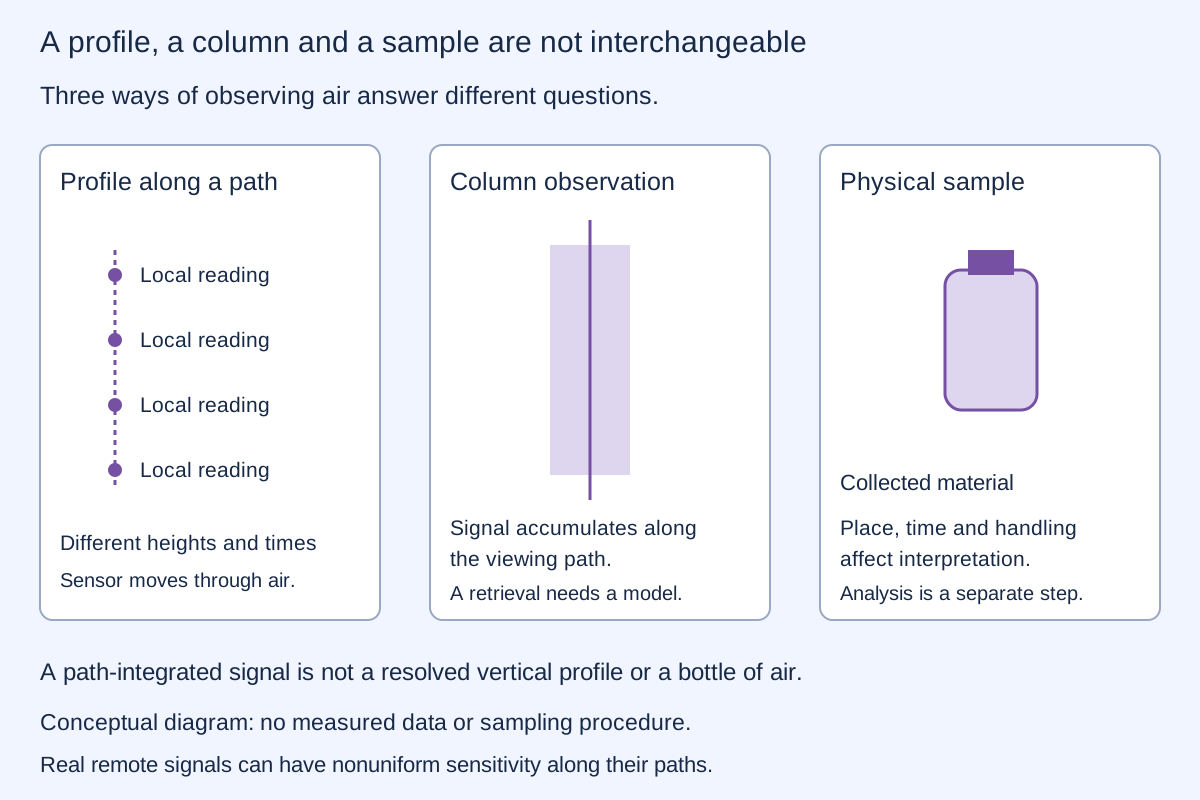
NOAA/NWS describes radiosonde measurements. Such instruments measure properties in situ; this does not imply they store physical samples of the atmosphere.
TWO INVENTED UNIFORM LAYERS · GEOMETRIC COLUMN ONLY
Each layer is 1 km thick. The lower layer's concentration changes; the upper layer compensates so their total column stays fixed. The substance and profiles are fictional. This is an arithmetic example, not a model of atmospheric chemistry.
The calculation is 1000 m×clower+1000m×cupper=2000mg/m²=2g/m². A column value alone cannot distinguish these profiles. A real remote instrument has wavelength-dependent weighting, path geometry and calibration; its signal is not automatically this simple integral. Additional measurements may help recover height information.
| Method | What is measured | What is not automatic |
|---|---|---|
| Ground-penetrating radar | Reflected electromagnetic signals and travel times | A depth without a speed model, or a unique material identity |
| Electrical resistivity | Electrical response to current flow | A chemical assay or a direct photograph |
| Seismic methods | Elastic-wave travel and response | A unique geological model from one signal |
Water, clay, salinity, geometry and material contrasts affect the response. A bright feature is not automatically a pipe, a leak or a known chemical composition. A USGS radar field study illustrates why penetration and interpretation depend on site conditions; one site's depth is not a universal instrument specification.
UNIFORM MEDIUM · VERTICAL TWO-WAY PATH
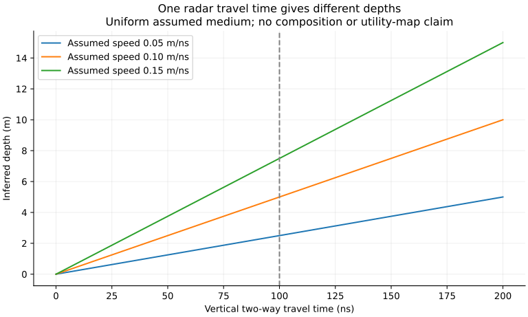
An echo goes down to a reflector and returns. Change the assumed signal speed while keeping the measured round-trip delay fixed. The inferred depth changes even though the delay does not.
A nanosecond (ns) is one billionth of a second. Using speed in m/ns and time in ns gives metres. The factor 2 accounts for the down-and-back path.
The model assumes zero instrument delay, known time origin, vertical travel and one uniform speed. Layering, oblique paths, refraction, wave attenuation and waveform interpretation are omitted. This is not a utility map or a guarantee that a buried object can be detected.
Cosmic muons can pass through substantial material. Measurements across directions, together with particle transport and detector models, can constrain how much material lies along those paths. A published muography study reconstructs hidden cavities; it does not validate every proposed particle scanner.
Neutrinos interact much more weakly at the energy used in the example below. Penetration is an advantage only if enough useful interactions can also be observed. A probability of interaction is not image resolution, chemical identification or a three-dimensional reconstruction.
CONDITIONAL NEUTRINO COUNT MODEL · NO INSTRUMENT DESIGN
Consider particles crossing an assigned rock column of density 2.7 g/cm³. The nominal cross section is 1.10×10−38cm² per nucleon, used as a representative charged-current value at about 1.1 GeV. The underlying iron measurement is being transferred approximately to generic rock, not treated as exact material-specific physics.
Nucleon column≈density×path length in centimetres×6.02214076×10²³ nucleons per gram. Optical depth τ is this column times cross section σ. Interaction probability is P=1−exp(−τ), evaluated numerically as −expm1(−τ) to avoid subtracting nearly equal numbers.
For assigned incident count N and detection efficiency η, mean detected count is λ=NPη. Independent rare events admit the Poisson approximation: relative count standard deviation 1/√λ and zero-event probability exp(−λ). With a fixed N and fixed per-particle probability, the exact count law is binomial; the tiny probabilities here justify the approximation. No background, correlations, detector saturation or uncertainty in N and η is included.
A mean below one does not forbid an event, and a mean of one does not guarantee an event. At zero expected count relative precision is undefined; the supplied controls use positive budgets and efficiencies. Very small displayed zero-event probabilities are numerical approximations, not guarantees.
The nominal measured cross section has a quoted uncertainty of 0.15×10−38cm². That uncertainty and target-composition transfer are not propagated into the displayed counting-only spread. Cross sections depend on energy, particle type, target and reaction. Natural muon imaging cannot be simulated by reusing this single neutrino cross section.
The Particle Data Group review provides the interaction context. The assigned particle budget has no source, beam, collection-time or detector geometry behind it. This chapter makes no fine-scanning or excavation claim.
Heating and nuclear transformation are different processes. Melting ordinary rock changes its physical state; it does not turn its nuclei into hydrogen. Any nuclear-conversion proposal would need its own reactions and matter/energy balance. No such mechanism is established here.
A REAL ASTRONOMY EXAMPLE · PUBLISHED ICECUBE ANALYSIS
For a five-year-old: IceCube does not take a picture of a tiny neutrino. Sometimes a neutrino bumps into something inside or near the detector and makes a fast-moving charged particle. That particle makes faint blue light in the ice. Many sensors record when the light arrives, and scientists check whether the pattern looks more like a real track or ordinary background.
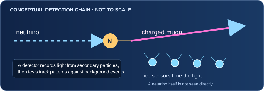
In a published search using IceCube data from 2011–2020, the collaboration tested 110 previously selected gamma-ray sources against expected atmospheric and diffuse-neutrino backgrounds. For NGC 1068, the analysis found an estimated excess of 79 events (statistical interval −20/+22) and a post-selection significance of 4.2σ. The authors interpreted this as evidence for TeV neutrino emission from that galaxy. The excess is a statistical estimate above modeled backgrounds, not 79 individually tagged neutrinos or a camera image of the source.
Why it matters: neutrinos can escape some dense cosmic environments that hide or absorb much of their light. Combining neutrino observations with telescopes that measure light can help researchers investigate how active galaxies accelerate particles. The result does not by itself settle every detail of the source's internal processes.
This modern published result illustrates the general idea of inferring neutrinos from secondary-particle signatures. It does not reconstruct or validate the brief secondhand historical claim in open idea 056: its earlier document is unavailable, and its detector, geometry, energy response, exposure, background method and provenance remain unknown.
IceCube Collaboration, Science 378 (2022), “Evidence for neutrino emission from the nearby active galaxy NGC 1068” · IceCube: muon-track reconstruction and atmospheric-background rejection.
A concentration tells us how much of a substance is present in a mixture. An emission rate describes how much leaves a source per unit time. Wind, mixing, flow and measurement geometry connect those questions.
A USGS study of volcanic-gas emission measurements explains the need for plume velocity in calculating emission rates. A concentration snapshot alone is insufficient. Temperature, pressure and whether concentration is reported on a wet or dry basis also matter when converting quantities.
An unexpected component may reflect the source, surrounding air or contamination. Repeated calibrated observations and independent context help distinguish them. A list of gases without measurements cannot establish a reservoir or working probe. No sampling, mixture or flame procedure is provided.
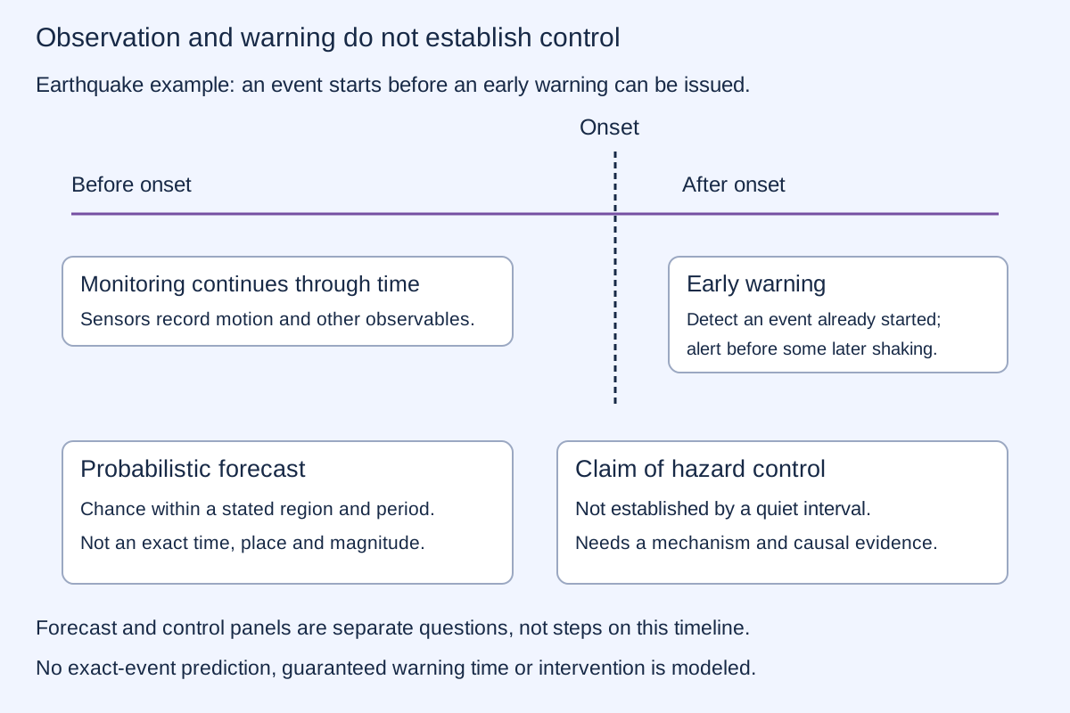
USGS distinguishes earthquake prediction from other monitoring products. A forecast assigns probabilities over defined regions and periods. Exact time, place and magnitude prediction is a different claim. This distinction does not imply that all hazard forecasts are impossible.
A quiet period after an alleged intervention is not by itself evidence that the intervention prevented an earthquake or eruption. A causal claim needs a mechanism, independent records, exposure information and a credible comparison with what otherwise might have happened. There is no hazard-prediction or fault/volcano-control tool in this chapter.
Today: atmospheric profiles support weather analysis; subsurface surveys support infrastructure and geological interpretation; emissions and ground-motion measurements support environmental decisions.
A possible next step: combine complementary calibrated observations with explicit uncertainty and models tested against independent evidence. More information can improve decisions without removing ambiguity or granting control over the environment.
REPRODUCIBLE IDEALIZED CALCULATIONS
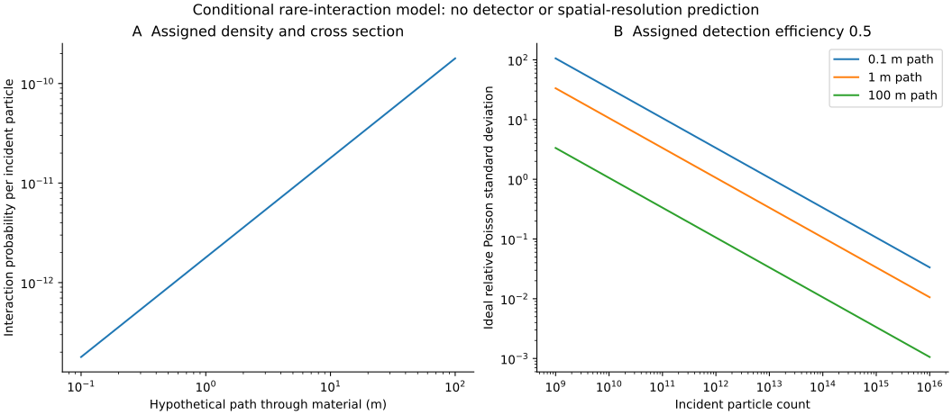
3,149 calculation rows: 603 radar cases, 101 particle columns, 2,424 count budgets and 21 constant-column profiles. No hazard probabilities or instrument performance are inferred from the number of cases.
Run the script with Python, NumPy and Matplotlib. Runtime and generator hash are recorded. Independent checks use SI unit conversions, a small-optical-depth series and direct layer integration. The stable probability calculation differs slightly from the earlier subtractive calculation, by about 3.64×10⁻⁶ relative at the two historical short paths; that numerical correction is not new experimental evidence.
These are assigned teaching models, not field measurements, a source-specific device test or a hazard forecast. Original project calculations remain unchanged; the clean probability calculation uses a numerically stable exponential expression.
Constructing a landscape, changing plant populations, observing animals and eliminating a pathogen are different interventions. Describing them together does not demonstrate a controlled ecosystem. Each claim needs a defined target, measurements of the intended change and checks for other effects. No such intervention or eradication result is supplied by this proposal.
ILLUSTRATIVE OCCUPANCY MODEL · ASSIGNED INPUTS ONLY
Simple version: Imagine a species lives in 40 of 100 woodland patches. If it hides well, one visit may miss it in many patches. More visits can reveal more of those same occupied places even though the real number of occupied places has not changed.
This simulation keeps 40 occupied sites fixed. Choose an assumed chance of detecting the species on one visit and the number of repeat visits. The curve shows the expected number of occupied sites where it has been detected at least once.
Rising line: expected occupied sites detectedFlat line: occupied sites in the fixed example
After 3 visits, the model expects to detect the species at 35.0 of the 40 occupied sites. About 5.0 occupied sites remain undetected in expectation. The assumed real occupancy stays at 40 sites.
Reading the picture: site occupancy asks whether the species is present at a place; abundance asks how many individuals are there. This simple simulation concerns occupancy only.
| Visits | Expected occupied sites detected | Expected occupied sites missed |
|---|---|---|
| 1 | 20.00 | 20.00 |
| 2 | 30.00 | 10.00 |
| 3 | 35.00 | 5.00 |
| 4 | 37.50 | 2.50 |
| 5 | 38.75 | 1.25 |
| 6 | 39.38 | 0.63 |
| 7 | 39.69 | 0.31 |
| 8 | 39.84 | 0.16 |
| 9 | 39.92 | 0.08 |
| 10 | 39.96 | 0.04 |
With independent visits and constant per-visit detection probability p, cumulative detection probability after k visits is 1 − (1 − p)k. Expected detected sites = 100 × 0.4 × [1 − (1 − p)k]. The model assumes occupancy stays fixed during this short survey, equal detectability at every occupied site, and no false-positive identifications. Real studies may need to account for observer, season, weather, habitat, survey effort, dependence and changing occupancy. This curve does not estimate abundance, a real species' status, or whether a conservation action caused a recovery.
The USGS North American Breeding Bird Survey data release (1966–2025) documents a standardized long-term bird survey: 50 stops per route, three minutes per stop, birds seen or heard, and one survey per route each year. Its records include survey conditions and observer information. Standardized data can help teams track trends and decide where further conservation work is needed; the counts are not a perfect census of every bird.
MacKenzie and colleagues' peer-reviewed occupancy study explains why not detecting a species does not prove it is absent when detection is imperfect, and shows how repeated surveys can help estimate occupancy. To decide whether protection helped, teams still need defined outcomes, monitoring over time and a justified comparison—not just more sightings.
Download the default expected values · Methods, assumptions and sources · Regenerate the CSV with Python · Model source · See the open idea and the information it lacks.
Finding a substance in an air sample would establish its presence under the sampling and measurement conditions. It would not show that nearby organisms require that substance to breathe. Explaining its source and its biological role are separate questions. An uncalibrated spectrum or a mistaken interpretation supplies neither answer.