Imagine this
This page looks at one kind of very high-energy light. A shield can change how much gets through. That alone cannot tell us if a person is safe.
THE FIELD GUIDE / 044 · RADIATION AND MATTER
A detector sees fewer photons behind an object. Some may have been absorbed; others may simply have changed direction. Understanding that difference helps us read measurements without drawing conclusions they cannot support.
Explore an idealized beam ↓This page looks at one kind of very high-energy light. A shield can change how much gets through. That alone cannot tell us if a person is safe.
Attenuation calculations help compare how a stated material changes a stated radiation beam. A shield might help in a defined setting after dose and exposure are measured.
This is an ideal calculation, not a safety certificate. The beam’s energy, shield shape, scattered light and a person’s exposure all matter.
Read-aloud starter; not yet tested with children. The fuller science, data, figures and sources follow below.
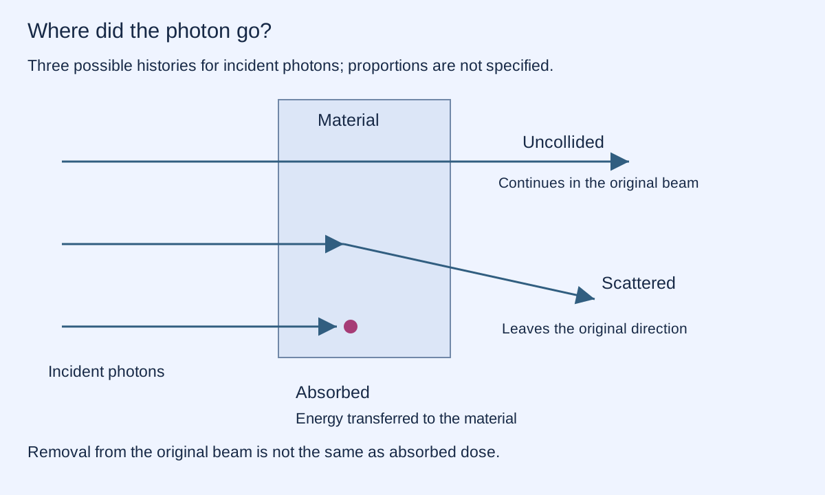
A photon is a packet of electromagnetic radiation. It may continue without interacting, scatter into another direction, or be absorbed in an interaction. Scattering can also transfer energy. Our drawing shows separate possible histories, not the percentages taking each path.
The NIST attenuation model describes a narrow beam whose photons initially have the same energy. Its interaction coefficient depends on energy and material. The exercise below uses only an assigned dimensionless depth, so it cannot tell you which material or thickness to choose.
ASSIGNED MATHEMATICAL EXAMPLE · NO EXPOSURE CALCULATION
Optical depth summarizes the amount of interaction along a path. It has no units. Increase it to see the fraction that reaches the end without an interaction. A depth of zero leaves the full original beam; each equal added depth multiplies the remaining fraction by the same factor.
“Removed” does not mean absorbed energy, destroyed radiation or avoided dose. The bar follows only the original, uncollided component. A very small positive fraction can be hard to see; the numerical result remains positive.
Set the depth of each layer. Under the same narrow-beam assumptions, their transmission factors multiply and their depths add.
T = exp(−τ), where T is the fraction of the initially uncollided beam and τ is optical depth. This solves dT/dτ = −T with T(0) = 1. For two layers, exp(−a) × exp(−b) = exp(−(a+b)). At τ = ln(2), exactly half the uncollided component remains.
The model does not track scattered-in photons, secondary particles, energy deposition, broad spectra, biological response or real detector geometry. Two real layers are not interchangeable for every radiation field just because their assigned depths sum to the same number. This is neither a protective-barrier design nor a safe-exposure calculation.
Ionizing radiation can affect DNA. But an effect that is physically possible is not a complete explanation of an observed population pattern. Each step below needs its own observations.
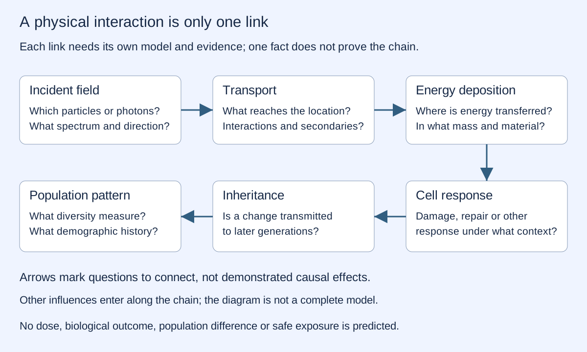
| Quantity | What it tells us |
|---|---|
| Incident field | Which particles arrive, with what energies, directions and rates. |
| Absorbed dose | Energy deposited per specified mass. One gray is one joule per kilogram. This is not a particle count or a tissue-weighted measure. |
| Cellular change | A defined molecular or cellular endpoint, with timing and measurement uncertainty. |
| Inherited variant | A change that is transmitted through reproduction; damage alone does not establish this. |
| Population pattern | Variant frequencies or diversity in a defined sample, influenced by many processes. |
An atmosphere can alter an incoming radiation field through interactions, including production of secondary particles. A calculation needs the incident particle types and energy spectrum, magnetic environment, atmospheric composition and column, and geometry. A single assigned photon curve cannot represent that whole process.
NASA's NAIRAS 3.0 model illustrates the broader task: it combines incident spectra, magnetic and atmospheric inputs with particle transport. This chapter does not run that model or estimate anyone's exposure.
Ancient radiation and present populations. Naming geological periods does not establish a radiation history. A proposed connection needs spectrum, intensity, geographic evidence, mutation signatures and population history. Migration, demography, selection and chance also affect diversity. Appearance, species counts and genetic diversity are different endpoints; social racial categories are not discrete genetic units or a biological hierarchy.
Gravity and neutron targeting. A neutron is electrically neutral and can respond to gravity. The neutron study by Nesvizhevsky and colleagues (2002) concerns a defined arrangement using Earth's gravity and a horizontal mirror. They do not demonstrate an unspecified artificial field steering individual neutrons toward moving reproductive cells. The proposal supplies no measured spatial uncertainty, feedback, deposited energy or outcome. A stated mutation count without a dataset is not a result.
Atmospheric shielding and inheritance. A reduced incoming component does not by itself predict inherited change or population uniformity. The transport calculation, tissue response, reproductive transmission and demographic explanation are separate missing links.
Studies with different species, exposure patterns and biological endpoints cannot be combined merely by dividing their dose values. An earlier arithmetic comparison in this project did only that unit-and-ratio exercise; it was not a transport or inheritance model and is not used in this simulation. A finding for one endpoint does not establish every possible effect; a null result does not establish universal impossibility.
Today: researchers use interaction models to interpret detector readings and compare well-defined measurements. Asking whether an instrument counts an original beam, scattered radiation or deposited energy prevents misleading comparisons.
Possible next step: an evidence dashboard could show transport assumptions, measurement uncertainty and missing biological links together. It could help teams identify which observation would distinguish competing explanations. Its usefulness depends on validated inputs; this simple curve cannot infer health, ancestry or protection.
REPRODUCIBLE MATHEMATICS AND PUBLISHED CALCULATIONS
PUBLISHED CALCULATION · MATERIAL-DEPENDENT EXAMPLE
Simple version: A fast proton is a tiny particle moving through plastic. This table estimates the average depth it reaches in one named kind of plastic before slowing down. It does not tell us whether a spacecraft, astronaut or person is safe.
The blue curve plots all 133 default proton energies returned by NIST PSTAR for its polyethylene preset. NIST reports projected range as average penetration depth along the particle’s starting direction. The main vertical axis keeps NIST’s published unit, grams per square centimetre. The centimetre values in the table divide this areal range by NIST’s stated polyethylene density, 0.94 g/cm³; they are equivalent average depths for that density.
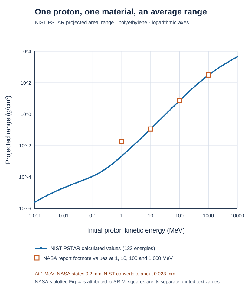
These are approximate text values from a report footnote, kept separate from the NIST table. The 1 MeV entries differ by a factor of about 8.8 after converting both to areal range with the report’s density. The original SRIM run settings and raw Figure 4 coordinates have not been recovered, so the discrepancy remains unresolved; it is not enough to declare either calculation wrong.
| Proton energy | NIST PSTAR projected range | Equivalent depth from NIST | NASA report footnote |
|---|---|---|---|
| 1 MeV | 0.002132 g/cm² | 0.023 mm | 0.2 mm |
| 10 MeV | 0.1131 g/cm² | 1.20 mm | 1.2 mm |
| 100 MeV | 7.235 g/cm² | 7.70 cm | 7.7 cm |
| 1,000 MeV | 308.1 g/cm² | 3.28 m | 330 cm |
Why this matters: Range calculations can help researchers decide which materials and thicknesses deserve more detailed spacecraft-radiation analysis. A single proton’s average range is only an early clue. Real space radiation contains many energies and particle types; materials can also create secondary particles. This graph calculates no radiation dose, health risk or protective performance.
There is no slider here: changing one proton’s energy could suggest a sharp pass/fail boundary or a safe thickness, neither of which this average-range calculation supports. The graph and comparison table show the published quantities behind this bounded calculation more honestly.
133 NIST points · CSVRetained NIST table · TXTParameters and source record · JSONMethods and limitsReproduce the figure · Python
Primary sources: NIST PSTAR tables · NIST quantities and methods · NIST projected-range definition · NIST polyethylene density and composition · NASA/TP-2020-220514, printed p. 4, Fig. 4 and footnotes 7–8. NIST data are reproduced with attribution; this derivative graph and the comparison are DMGB Systems’ presentation, not a NIST or NASA endorsement.
Calculations are from the NIST PSTAR online table retrieved 29 September 2026, standard energy grid, material preset Polyethylene (material 221), retained unchanged. Depth conversion uses 0.94 g/cm³. The NASA report values are quotations from its footnote, not raw beam measurements. This comparison does not reproduce or validate NASA Figure 4.
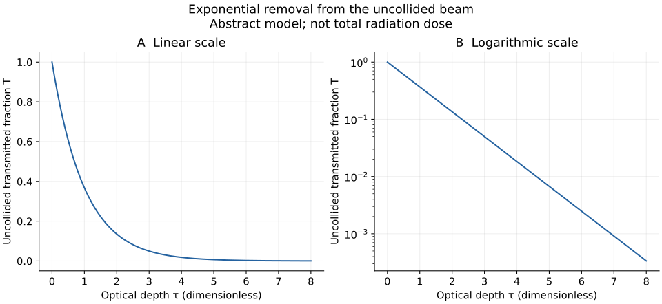
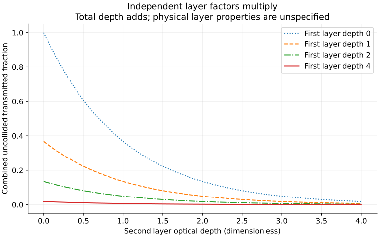
The study exports 801 single-depth rows at steps of 0.01 and 1,681 layer pairs at steps of 0.1: 2,482 rows in total. These are computed values, not measurements; no confidence bands are invented.
Single-depth CSV · Layer-pair CSV · Standalone reproduction script · Methods and limits · Parameters and runtime · Numerical checks · Independent CSV check
Run the script with Python, NumPy and Matplotlib. Checks cover zero and half-transmission limits, monotonicity, complementary fractions, layer multiplication, invalid inputs and an independent numerical integration of the differential equation. The integration error falls by about four when the step size halves, as expected for the method. Agreement checks this mathematical construction, not a physical shielding system.